IDEEA: Electric power sector model

Configuration

Set the base year (BY), the number of regions (5 or 32), and other spatial configuration.

base_year <- 2019 # the first year of the model (base year or `BY`)

# Currently '5' and '32' are available
nreg <- 32
# nreg <- 5

offshore <- TRUE # should offshore regions be included
islands <- TRUE # should islands be included

Set transmission matrix for the model. The current matrix is used for the 5-region model, and the newlines_v0X matrix is used for the 32-region model. The newlines_v01 matrix has ~70 power lines, newlines_v02 has ~30 power lines, and newlines_v03 has ~50 power lines. See details in the vignette("transmission").

if (nreg == 5) {
  transmission_matrix <- "current"
} else if (nreg == 32) {
  # transmission_matrix <- "newlines_v01" # ~70 power lines
  # transmission_matrix <- "newlines_v02" # ~50 power lines
  transmission_matrix <- "newlines_v03" # ~30 power lines
} else {
  stop("Only 5 and 32 regions are currently implemented")
}

Set parameters for intermittent renewable energy sources (wind and solar) and land use assumptions.

# wind turbine hub height
win_hub_height <- 100 # meters, hub height, options:  50, 100, 150 

# land use for wind farms
win_max_land_use <- 0.25 # % of the land area
# land requirements assumption for wind farms, adjusted for maximum land use
win_onshore_max_MW_km2 <- 20 * win_max_land_use # 20 MW/km2 * % of land use
win_offshore_max_MW_km2 <- 5 * win_max_land_use # 5 MW/km2 * % of land use
# the range is ~6-50 MW/km2 see: 
# https://web.stanford.edu/group/efmh/jacobson/Articles/I/WindSpacing.pdf
# https://www.nrel.gov/docs/fy09osti/45834.pdf, p.18

# land use for solar farms
sol_max_land_use <- 0.1 # % of the land area
sol_onshore_max_MW_km2 <- 40 * sol_max_land_use
# sol_offshore_max_MW_km2: 0 * sol_max_land_use # not implemented
# ~40 MW/km2 (40 GW/1000km2)
# see: https://www.nrel.gov/docs/fy19osti/72399.pdf, p.18
# convert("ha/MW", "km2/MW", 40) 

Adjust wind and solar capacity factors clustering tolerance (from 0 to 1). The clustering process is based on correlation of the capacity factors between MERRA2 cells (see details on merra2ools. The lower value gives more clusters per region, and larger regions’ area will have more clusters and may require higher values to reduce the number of clusters.

if (nreg == 5) {
  tol_win_cl <- 0.10
  tol_sol_cl <- 0.05
} else if (nreg == 32) {
  tol_win_cl <- 0.05
  tol_sol_cl <- 0.02
} else {
  stop("Only 5 and 32 regions are currently implemented")
}

# region variable name to use in functions (e.g. `get_ideea_data`)
regN <- paste0("reg", nreg)
regN_off <- paste0(regN, "_off")

library(tidyverse)
library(data.table)
library(sf)
library(glue)
library(data.table)
library(here)
library(IDEEA)
set_progress_bar()
# show_progress_bar(F)

If not done yet, configure your system, editing and saving global options:

ideea_global_options(edit = TRUE)

Regions

ideea_sf <- get_ideea_map(nreg,
  offshore = offshore, islands = islands,
  rename = FALSE
)
plot(ideea_sf[regN_off], key.width = lcm(4.5))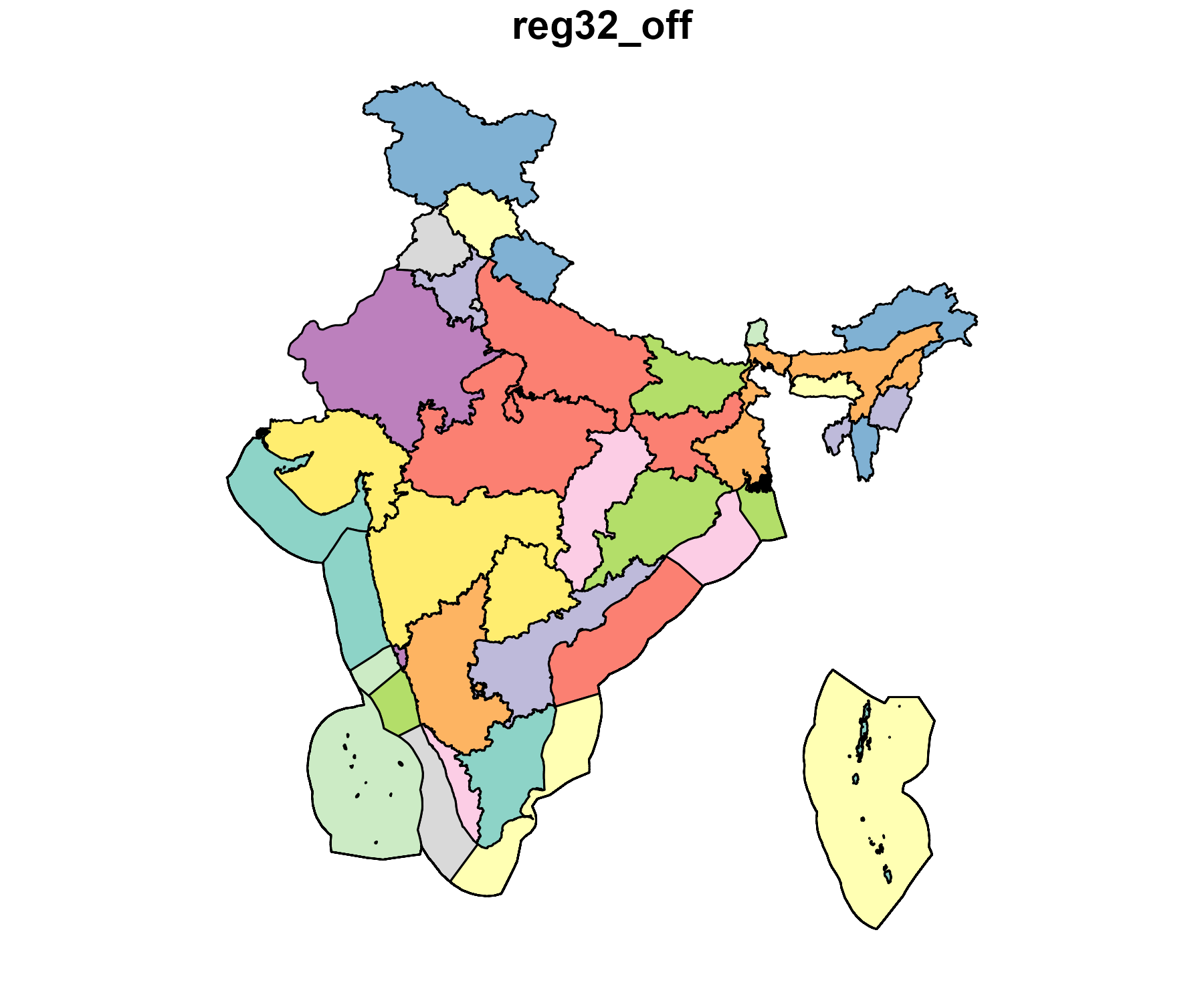

Time resolution

Structure of sub-annual time resolution is done calendar objects, that specifies levels of nested time-frames (such as ‘ANNUAL’, ‘MONTH’, ‘DAY’, ‘HOUR’, etc. depending on the modeling goals and decided level of details). This structure of modeled sub-annual time resolution is assigned by a timetable data.frame with columns named as used time-frames, as well as ‘slice’ (refers to the lowest level of ‘time-slices’ with unique names, e.g. ‘d001_h15’ indicating the 1st day of the year and the 15th hour of the day), the ‘share’ column (for the share of the time-frame in the year), and ‘weight’ (for the weight of the time-frame in the year, used in sampled calendars).

# timetable with 3 levels of timeframes: ANNUAL, YDAY, HOUR
ideea_modules$calendars$calendar_d365_h24@timetable
#>       ANNUAL   YDAY   HOUR    slice        share weight
#>       <char> <char> <char>   <char>        <num>  <num>
#>    1: ANNUAL   d001    h00 d001_h00 0.0001141553      1
#>    2: ANNUAL   d001    h01 d001_h01 0.0001141553      1
#>    3: ANNUAL   d001    h02 d001_h02 0.0001141553      1
#>    4: ANNUAL   d001    h03 d001_h03 0.0001141553      1
#>    5: ANNUAL   d001    h04 d001_h04 0.0001141553      1
#>   ---                                                  
#> 8756: ANNUAL   d365    h19 d365_h19 0.0001141553      1
#> 8757: ANNUAL   d365    h20 d365_h20 0.0001141553      1
#> 8758: ANNUAL   d365    h21 d365_h21 0.0001141553      1
#> 8759: ANNUAL   d365    h22 d365_h22 0.0001141553      1
#> 8760: ANNUAL   d365    h23 d365_h23 0.0001141553      1

This time-table is to define a calendar object, that also describes the hierarchy of time-frames and sets the sequence of the time-slices.

# the model is defined with the full calendar
calendar_d365_h24 <- ideea_modules$calendars$calendar_d365_h24

# a scenario can be run with a subset of the time-slices
calendar_d365_h24_subset <-
  ideea_modules$calendars$calendar_d365_h24_subset_1day_per_month

The model object (described below) must have the calendar object with all time-frames and time-slices used in the model. However, scenarios can be solved for a subset of the time-slices, defined by another calendar object with sub-set of time-slices. Here we define a calendar with a subset of 1 day per month and 24 hours per each day. Therefore, the total number of time-slices in the subset is 12 days * 24 hours = 288 time-slices (vs. 8760 time-slices in the full calendar).

Commodities

Commodities are the main objects of the model, representing the goods and services that are traded in the model. Commodities can be energy carriers (e.g. electricity, coal, oil, gas, biomass), emissions (e.g. CO2, NOx, SOx, PM), or other goods and services. Commodities are defined by their name, description, unit of measure, and time-frame by the newCommodity function. Some of the commodity-objects are pre-built in the energy module, and can be loaded from there. Commodities specific to the electricity model are defined below. Important features of commodities are their time-frame, and the limit type (slot @limtype) that defines the balance equation for the commodity. By default the limit type is set to “LO” (lower bound) meaning that excess of commodity is allowed, but the deficit is not. Other options are “UP” (upper bound) and “FX” (equality).

# energy
ELC <- newCommodity(
  name = "ELC",
  desc = "Electricity",
  unit = "GWh",
  timeframe = "HOUR"
)

# emissions
CO2 <- newCommodity(
  name = "CO2",
  desc = "Carbon emissions",
  unit = "kt",
  timeframe = "ANNUAL"
)

NOX <- newCommodity(
  name = "NOX",
  desc = "Nitrogen oxide emissions NOx",
  unit = "kt",
  timeframe = "ANNUAL"
)

SOX <- newCommodity(
  name = "SOX",
  desc = "Sulfur oxide emissions SOx",
  unit = "kt",
  timeframe = "ANNUAL"
)

PM <- newCommodity(
  name = "PM",
  desc = "Particulate matter (particle pollution)",
  unit = "kt",
  timeframe = "ANNUAL"
)

REN <- newCommodity(
  name = "REN",
  desc = "Generic renewable energy",
  unit = "GWh",
  timeframe = "ANNUAL"
)

# storing commodities in a repository
repo_comm <- newRepository(
  name = "repo_comm",
  desc = "Electricity & emissions commodities"
) |>
  add(ELC, CO2, NOX, SOX, PM)

Demand options

For the electricity-only model, the electricity is considered as the final product, and the final demand can be set exogenously via the demand class. The newDemand function creates an object of class demand with detailed representation of the demanded electricity by region, time-slice, and year. The values of demand without information on the parameter dimension, such as the region, time-slice, or year are considered default for the non-specified dimensions, and will be filled-in on the interpolation step of the model along with the missing years. Therefore it is enough to set values for the base-year and the last year, if the demand is expected to grow linearly. The load curve by region in India for 2019 is stored in the load_2019_MWh dataset, and used in this example as the base-year demand, extrapolated through the model’s horizon.

# call the load curve by region in 2019 from IDDEA dataset
load_BY <- get_ideea_data("load_2019_MWh", nreg = nreg, variable = "MWh") |>
  mutate(GWh = MWh / 1e3) |>
  select(-MWh)
# rename(region = {{regN}})

# define `demand` object with the historical load curve
DEMELC_BY <- newDemand(
  name = "DEMELC_BY",
  desc = "Houlry electric demand by region, base-year level",
  commodity = "ELC",
  unit = ELC@unit,
  dem = data.frame(
    region = load_BY[[regN]],
    # year = load_BY$year, # assign to all years
    slice = load_BY$slice,
    dem = load_BY$GWh # * dem_adj
  )
)

# display first 6 regions
ggplot(filter(load_BY, get(regN) %in% unique(load_BY[[regN]])[1:6])) +
  geom_line(aes(HOUR, GWh, color = YDAY, group = YDAY), alpha = .25) +
  scale_color_viridis_c(option = "H", limits = c(1, 365)) +
  scale_x_continuous(limits = c(0, 23)) +
  # facet_wrap(~ get(regN), ncol = floor(nreg / 3), scales = "free_y") +
  facet_wrap(~ get(regN), ncol = 2, scales = "free_y") +
  labs(y = "GWh", x = "hour") +
  theme_bw()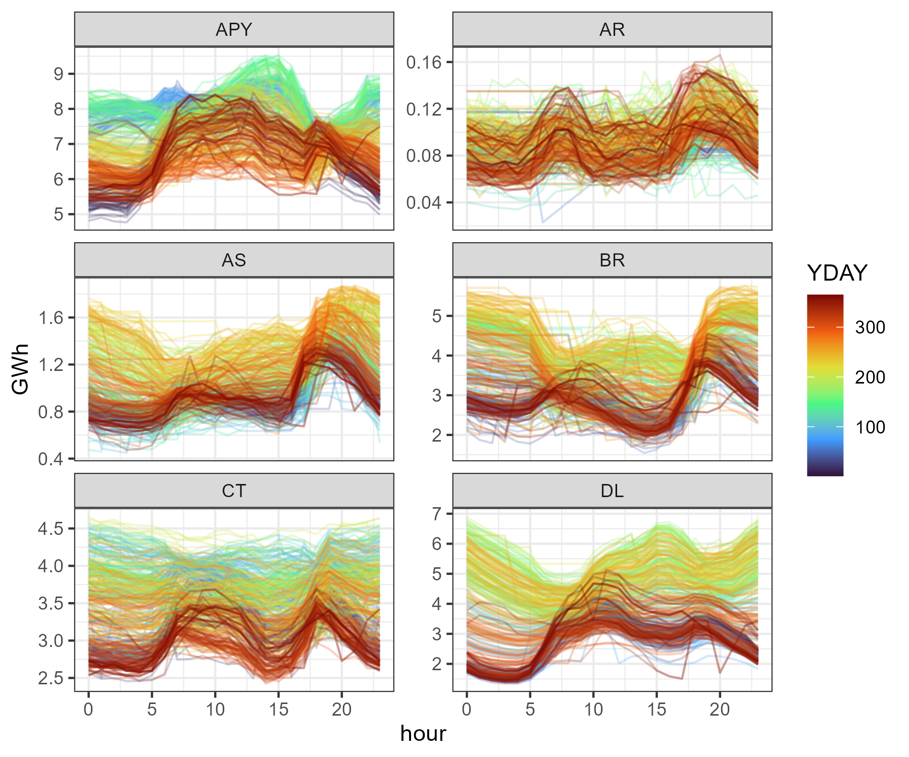

Hourly load by region, 2019 (first six regions)

ggsave(glue("load_2019_{regN}.png"), width = 7, height = 9, path = "tmp")

The demand growth is set by another demand-object with linear growth of the demand in every region, time-slice from zero to 2x the base-year level by 2050, and 3x by 2070. If the model horizon is longer, the demand can be extrapolated further.

# define demand in several years, e.g. 2020, 2050, 2070,
# which will be interpolated before solving the model ('interpolation' step)
load_2x_2050 <-
  rbind(
    mutate(load_BY, year = 2020, GWh = 0.0 * GWh),
    mutate(load_BY, year = 2050, GWh = 2 * GWh),
    mutate(load_BY, year = 2070, GWh = 3 * GWh)
  ) |>
  as.data.table()
load_BY
#>          reg32 offshore mainland    slice            datetime MONTH  YDAY  HOUR
#>         <char>   <lgcl>   <lgcl>   <char>              <POSc> <int> <int> <int>
#>      1:    APY    FALSE     TRUE d001_h00 2019-01-01 00:00:00     1     1     0
#>      2:    APY    FALSE     TRUE d001_h01 2019-01-01 01:00:00     1     1     1
#>      3:    APY    FALSE     TRUE d001_h02 2019-01-01 02:00:00     1     1     2
#>      4:    APY    FALSE     TRUE d001_h03 2019-01-01 03:00:00     1     1     3
#>      5:    APY    FALSE     TRUE d001_h04 2019-01-01 04:00:00     1     1     4
#>     ---                                                                        
#> 262796:     WB    FALSE     TRUE d365_h19 2019-12-31 19:00:00    12   365    19
#> 262797:     WB    FALSE     TRUE d365_h20 2019-12-31 20:00:00    12   365    20
#> 262798:     WB    FALSE     TRUE d365_h21 2019-12-31 21:00:00    12   365    21
#> 262799:     WB    FALSE     TRUE d365_h22 2019-12-31 22:00:00    12   365    22
#> 262800:     WB    FALSE     TRUE d365_h23 2019-12-31 23:00:00    12   365    23
#>              GWh
#>            <num>
#>      1: 5.468734
#>      2: 5.494523
#>      3: 5.349227
#>      4: 5.302847
#>      5: 5.624311
#>     ---         
#> 262796: 5.776000
#> 262797: 5.580000
#> 262798: 5.278000
#> 262799: 4.845000
#> 262800: 4.554000

# define the second demand object with the load growth
DEMELC_2X <- newDemand(
  name = "DEMELC_2X",
  desc = "Additional demand growth, proportional to the current load",
  commodity = "ELC",
  unit = ELC@unit,
  dem = data.frame(
    region = load_2x_2050[[regN]],
    year = load_2x_2050$year,
    slice = load_2x_2050$slice, # comment to assign to all hours
    dem = load_2x_2050$GWh # * dem_adj
  )
)

Alternative demand-objects can be created and added to the model before interpolation/solution to represent different scenarios or policy options.
Another ways to set the demand in the model also available. For example, export objects define the potential external demand with levels and also the price of the electricity. If other sectors are modeled, they can also set the demand for electricity, e.g. transport or industry modules.

Supply & resources

While demand objects set the final demand commodity (ELC in this example), the supply objects define the sources of primary commodities (e.g. coal, gas, oil, biomass, nuclear, renewable energy sources) that are used in the production of the final or interim products. The resources used in the electricity model has been already defined in the energy module, and can be loaded from there. Another way to introduce a supply of a commodity to the model is import from another region or from outside the model regions (“The Rest of the World”, ROW). For every tradable energy commodity we defined the import with higher than domestic supply price to ensure that the domestic supply is used first and extend the availability of the commodities’ supply beyond the domestic resources – essencial for long-term planning.

Primary energy

# import energy supply module
energy_module <- ideea_modules$energy[[regN]]

# check if the module is available for the requested number of regions
if (is_empty(energy_module)) {
  stop("ideea_modules$energy is not available for ", nreg, " regions")
}

# define repository for energy supply and resources
repo_supply <- newRepository(
  name = "repo_supply",
  desc = "Energy supply (markets)"
) |>
  add( # import objects from energy module
    # coal
    energy_module$COA, # coal commodity
    energy_module$SUP_COA, # coal domestic supply
    energy_module$IMP_COA, # coal import
    # natural gas
    energy_module$GAS, # natural gas commodity
    energy_module$SUP_GAS, # natural gas domestic supply
    energy_module$IMP_GAS, # natural gas import
    # oil
    energy_module$OIL, # oil commodity
    energy_module$SUP_OIL, # oil domestic supply by region
    energy_module$IMP_OIL, # oil import
    # biomass
    energy_module$BIO, # biomass commodity
    energy_module$RES_BIO, # domestic resource of biomass
    # nuclear
    energy_module$NUC, # nuclear fuel commodity
    energy_module$IMP_NUC, # Nuclear fuel international market
    # CCS storage potential (separate repo, see below)
    # energy_module$CO2SINK, # stored CO2 commodity
    # energy_module$RES_CO2SINK, # CO2 storage potential
    #
    REN, # all type of non-fuel (renewable) energy
    newSupply(
      name = "RES_REN",
      commodity = "REN",
      desc = "An artificial commodity to represent all renewable energy"
    ),
    overwrite = F # restrict duplicate objects
  )

# check
summary(repo_supply)
#> commodity    import    supply 
#>         6         4         5
names(repo_supply)
#>  [1] "COA"     "SUP_COA" "IMP_COA" "GAS"     "SUP_GAS" "IMP_GAS" "OIL"    
#>  [8] "SUP_OIL" "IMP_OIL" "BIO"     "RES_BIO" "NUC"     "IMP_NUC" "REN"    
#> [15] "RES_REN"

Land

Land resources for solar and wind farms are defined via supply classes along with solar and wind technologies (see ‘Generating technologies’ section below).

Carbon storage

The geological potential for carbon storage by region is defined in CCUS document, stored in IDEEA modules.

# import CCS potential from energy supply module

repo_geoccs <- newRepository(
  name = "repo_ccs",
  desc = "Carbon storage potential by region",
  # CCS storage potential
  energy_module$CO2SINK, # stored CO2 commodity
  energy_module$RES_CO2SINK # CO2 storage potential
)
summary(repo_geoccs)
#> commodity    supply 
#>         1         1

# clean-up
rm(energy_module)

Capacity factors

The availability of renewable energy sources (solar, wind, hydro) is defined by the capacity factors (CF) that represent the share of the potential energy that can be harvested in a given time-frame per unit of a generator capacity. The capacity factors are defined by the weather objects with the time-frame of the weather data (e.g. “HOUR” for hourly data, “YDAY” for daily data). The weather data can be obtained from the external sources (e.g. NREL, MERRA2, ERA5), some are saved in the IDEEA datasets. The capacity factors can be defined for the whole region, or for the specific locations.

Solar

This example implements the solar capacity factors for the regions of India, based on the MERRA2 dataset. The capacity factors are defined for the tilted tracking system (tl), estimated with merra2ools package.

# get clustered capacity factors from `ideea_extra` dataset
# if the data with requested parameters is not pre-saved, 
# it will be calculated from the raw MERRA2 data using `merra2ools` package
# and cashed in the `ideea_extra` dataset
solar_cf <- get_ideea_cf("sol", nreg = nreg, year = 2019, tol = tol_sol_cl)
#> Reading capacity factors data from:
#>    D:/Dropbox/projects/ideea_extra//merra2/cf_sol_r32_TOL02_d365_h24_2019.fst 
#>    Maximum number of clusters per region: 8
# get map of solar clusters
ideea_sol_cl_sf <- get_ideea_cl_sf("sol", nreg = nreg, tol = tol_sol_cl) |>
  mutate(
    # create/update MW_max based on land use assumptions 
    MW_max = if_else(!offshore, sol_onshore_max_MW_km2 * as.numeric(area), 0)
  )

# filter out offshore regions
solar_cf <- solar_cf |>  
  filter(!grepl("_off$", solar_cf[[regN_off]])) |>
  unique()
solar_cf$cluster |> unique()
#> [1] 1 2 3 4 5 6 7 8

# maximum number of clusters:
sol_clust_max <- max(solar_cf$cluster) 
sol_clust_digits <- max(nchar(sol_clust_max), 2)

# add column with commodity name for the cluster's land
ideea_sol_cl_sf <- ideea_sol_cl_sf |>
  mutate(land_comm = name_with_cluster(
    "LAND_SOL_CL", cluster, ndigits = sol_clust_digits))

# create repository to store solar capacity factors (weather objects)
WSOL <- newRepository(name = "Solar capacity factors")

# create weather object for every cluster in a loop and store in the repository
for (i in unique(solar_cf$cluster)) {
  # select data for the cluster
  x <- filter(solar_cf, cluster == i)
  # create weather object
  WSOL_i <- newWeather(
    name = name_with_cluster("WSOL_CL", i, ndigits = sol_clust_digits),
    desc = name_with_cluster(
      "Solar capacity factors, tilted tracking system (tl), cluster ", i
    ),
    region = unique(x[[regN]]),
    timeframe = "HOUR",
    weather = data.frame(
      region = x[[regN]],
      slice = x$slice,
      # year = NA # all years
      wval = x$scf_tl
    )
  )
  # add weather object to the repository
  WSOL <- add(WSOL, WSOL_i)
  # clean-up
  rm(x, WSOL_i)
}

# check the repository
summary(WSOL) 
#> weather 
#>       8
names(WSOL) |> head()
#> [1] "WSOL_CL01" "WSOL_CL02" "WSOL_CL03" "WSOL_CL04" "WSOL_CL05" "WSOL_CL06"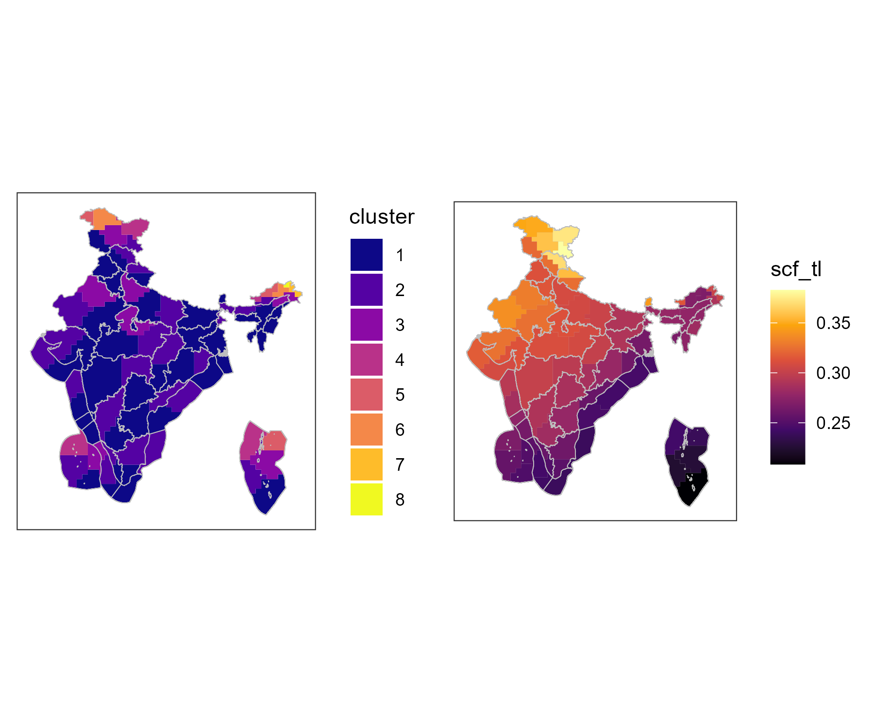

Solar clusters and average solar capacity factors by cluster, tilted tracking system (tl)

Wind

The wind capacity factors are defined for the regions of India, based on the MERRA2 dataset. The capacity factors are estimated for the 100m height (wcf100m) with merra2ools package, the data for 5 regions is saved in ideea_data.

# get clustered capacity factors from `ideea_extra` dataset
wind_cf <- get_ideea_cf("win", nreg = nreg, year = 2019, tol = tol_win_cl)
#> Reading capacity factors data from:
#>    D:/Dropbox/projects/ideea_extra//merra2/cf_win_r32_TOL05_d365_h24_2019.fst 
#>    Maximum number of clusters per region: 12
# get map of wind clusters
ideea_win_cl_sf <- get_ideea_cl_sf("win", nreg = nreg, tol = tol_win_cl) |>
  # update MW_max based on land use assumptions
  mutate(
    MW_max = if_else(offshore, 
                     win_offshore_max_MW_km2 * as.numeric(area),
                     win_onshore_max_MW_km2 * as.numeric(area)
                     )
    )

# maximum number of clusters:
win_clust_max <- max(wind_cf$cluster) 
win_clust_digits <- max(nchar(win_clust_max), 2)

# add column with commodity name for the cluster's land
ideea_win_cl_sf <- ideea_win_cl_sf |>
  mutate(
    land_comm = name_with_cluster(
      if_else(offshore, "LAND_WIF_CL", "LAND_WIN_CL"),
      cluster, ndigits = win_clust_digits)
  )

Notation: WIN - onshore wind WIF - offshore wind WIND - both, onshore and offshore wind

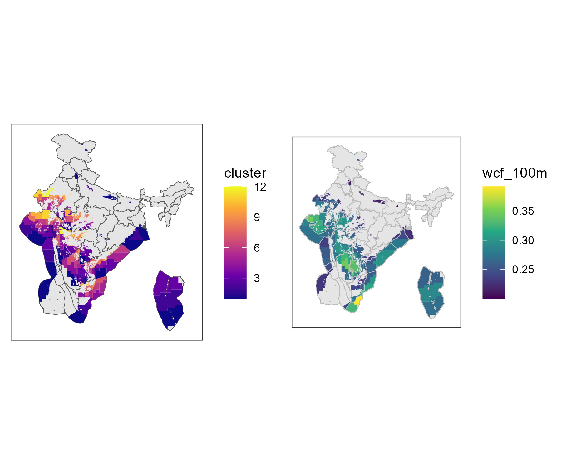
Wind clusters and average wind capacity factors by cluster, 100m height

Onshore

# repository to store onshore wind capacity factors (weather objects)
WWIN <- newRepository(name = "Onshore wind capacity factors")

# create weather object for every cluster in a loop and store in the repository
for (i in unique(wind_cf$cluster)) {
  x <- filter(wind_cf, cluster == i, !grepl("_off", wind_cf[[regN_off]]))
  # stop()
  if (nrow(x) == 0) next
  WWIN_i <- newWeather(
    name = name_with_cluster("WWIN_CL", i, ndigits = win_clust_digits),
    desc = name_with_cluster(
      "Onshore wind 100m height capacity factors, cluster ", i
    ),
    region = unique(x[[regN]]),
    timeframe = "HOUR",
    weather = data.frame(
      region = x[[regN]],
      slice = x$slice,
      # year = NA # all years
      wval = x$wcf_100m
    )
  )
  WWIN <- add(WWIN, WWIN_i)
  rm(x, WWIN_i)
}

# Check the repository
summary(WWIN)
#> weather 
#>      12
names(WWIN) |> head()
#> [1] "WWIN_CL01" "WWIN_CL02" "WWIN_CL03" "WWIN_CL04" "WWIN_CL05" "WWIN_CL06"

Offshore

# repository to store offshore wind capacity factors (weather objects)
WWIF <- newRepository(name = "Offshore wind capacity factors")

# create weather object for every cluster in a loop and store in the repository
for (i in unique(wind_cf$cluster)) {
  x <- filter(wind_cf, cluster == i, grepl("_off", wind_cf[[regN_off]]))
  if (nrow(x) == 0) next
  # stop()
  WWIF_i <- newWeather(
    name = name_with_cluster("WWIF_CL", i, ndigits = win_clust_digits),
    desc = name_with_cluster(
      "Offshore wind 100m height capacity factors, cluster ", i, 
      ndigits = win_clust_digits
    ),
    region = unique(x[[regN]]),
    timeframe = "HOUR",
    weather = data.frame(
      region = x[[regN]],
      slice = x$slice,
      # year = NA # all years
      wval = x$wcf_100m
    )
  )
  WWIF <- add(WWIF, WWIF_i)
  rm(x, WWIF_i)
}

# Check the repository
summary(WWIF)
#> weather 
#>       7
names(WWIF) |> head()
#> [1] "WWIF_CL01" "WWIF_CL02" "WWIF_CL03" "WWIF_CL04" "WWIF_CL05" "WWIF_CL06"
# WWIF@data$WWIF_CL01

Hydro

The hydro capacity factors are based on the official country-wide hourly data for India in 2013. This simplification is used to demonstrate the model’s capabilities and can be replaced with more detailed data if available.

# The data is stored in the IDEEA package dataset
# ideea_data$hydro_hourly_cf_2013 - raw data
hydro_cf <- get_ideea_data("hydro_hourly_cf_2013", raw = TRUE) |>
  mutate(slice = dtm2tsl(datetime), .after = "datetime")

WHYD <- newWeather(
  name = "WHYD",
  desc = "Hydro CUF",
  timeframe = "HOUR",
  weather = data.frame(
    # region = NA, # same for all regions
    slice = hydro_cf$slice,
    # year = NA # same for all years
    wval = hydro_cf$cf
  )
)

Generating technologies

The pre-existing capacity of power generation can be defined as groups of technologies, aggregated by the primary fuel type and other technological features, such as the efficiency, the costs, the lifetime, emissions, etc. In this example we use open-source datasets from WRI with some up-to-date corrections to represent the existing capacity of the power plants in India by the model regions and primary fuels. While the capacity is taken from the open WRI dataset, the technology parameters are collected by the IDEEA group, and have been used to define technology objects in the techs module (ideea_modules$techs).

# get WRI data for the existing capacity, aggregated by region and primary fuel
cap_0 <- get_ideea_data(
  name = "generators_wri",
  variable = c("primary_fuel", "capacity_mw"),
  nreg = nreg
) |>
  filter(capacity_mw > 0) # drop zeros

# get updated summary data for selected fuel type, 2020, aggregated by region
cap_1 <- get_ideea_data(
  name = "generators_2020",
  nreg = nreg,
  variable = c("Solar", "Wind", "Biomass", "Small Hydro")
) |>
  # reshape the table in long format
  pivot_longer( 
    cols = any_of(c("Solar", "Wind", "Biomass", "Small Hydro")),
    names_to = "primary_fuel",
    values_to = "capacity_mw"
  )  

# combine the datasets (updating WRI data with the newer capacity of renewables)
cap <- bind_rows(
  filter(cap_0, !grepl("Solar|Wind|Biomass", primary_fuel)),
  cap_1
) |>
  # add_reg_off(regN = regN) |>  
  group_by(across(any_of(
    c(regN, regN_off, "offshore", "primary_fuel")
  ))) |>
  summarize(capacity_mw = sum(capacity_mw, na.rm = T), .groups = "drop") |>
  as.data.table()

cap_sf <- ideea_sf |>
  right_join(cap) |>
  filter(!is.na(primary_fuel), capacity_mw > 10)
#> Joining with `by = join_by(offshore, reg32)`

a <- ggplot() +
  geom_sf(data = ideea_sf, fill = "grey") +
  geom_sf(aes(fill = capacity_mw / 1e3), data = cap_sf) +
  scale_fill_viridis_c(option = "H", name = "GW", trans = "identity") +
  facet_wrap(~primary_fuel) +
  theme_bw() +
  theme(
    # panel.background = element_rect(fill = "aliceblue"),
    # panel.grid = element_line(color = "white", size = 0.8),
    axis.ticks = element_blank(),
    axis.text = element_blank()
  )
# a
ggsave("tmp/installed_capacity.png", a,
  width = 6, height = 7,
  scale = 1.25
)
try(a)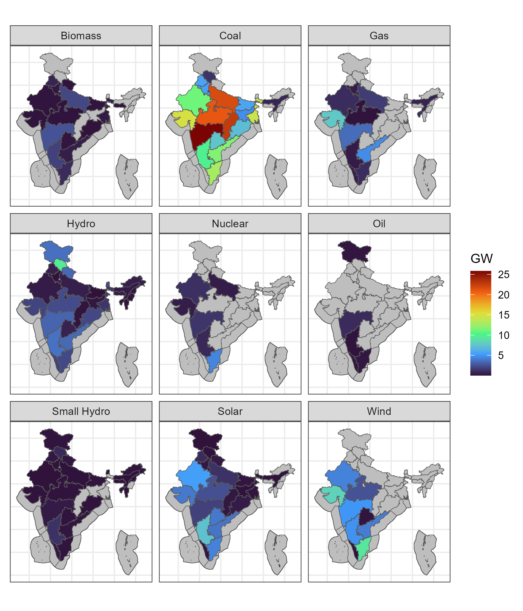

Existing capacity maps (WRI, 2021)

cap$primary_fuel |> unique()
#> [1] "Biomass"     "Hydro"       "Small Hydro" "Solar"       "Wind"       
#> [6] "Coal"        "Gas"         "Nuclear"     "Oil"

# summary table
cap |>
  group_by(primary_fuel, offshore) |>
  summarize(capacity_GW = sum(capacity_mw) / 1e3, .groups = "drop") |>
  arrange(desc(capacity_GW)) |>
  knitr::kable(
    caption = "Installed capacity by primary fuel type in 2020"
    )

Installed capacity by primary fuel type in 2020

primary_fuel	offshore	capacity_GW
Coal	FALSE	204.91922
Hydro	FALSE	45.56147
Wind	FALSE	38.61986
Solar	FALSE	37.46462
Gas	FALSE	24.94751
Biomass	FALSE	10.23201
Nuclear	FALSE	8.78000
Small Hydro	FALSE	4.60707
Oil	FALSE	1.68084

Coal-fired

There are several generations of coal-fired power plants, from sub-critical to supercritical, and ultra-supercritical, with different efficiencies, costs, and emissions. The existing capacity (stock) of coal-fired power plants in this example is assumed to be represented by the ECOASUP technology with average efficiency, which will linearly retire by 2040. More advanced technologies (ECOAULT) by vintages (2020, 2030, 2040, 2050) are available for investment. The technology with carbon capture is defined the the CCS section below.

# Existing capacity
cap_coa <- cap |>
  filter(grepl("Coal", primary_fuel)) |>
  filter(!offshore) |>
  mutate(year = 2020, .before = 1)

# assume age-based retirement of 2020 capacity by 2030 is 20%
cap_coa_2030 <- cap_coa |>
  mutate(year = 2030, capacity_mw = 0.8 * capacity_mw)

# assume further retirement of 2020 capacity by 2040 is 90%
cap_coa_2040 <- cap_coa |>
  mutate(year = 2040, capacity_mw = 0.1 * capacity_mw)

# combine
cap_coa <- cap_coa |>
  bind_rows(cap_coa_2030) |>
  bind_rows(cap_coa_2040)
# Note: the existing capacity will be linearly interpolated from 2020 to 2040
# cap = 0 after 2040

# load coal technology (assume Super-critical for all existing capacity)
ECOASUP_2020 <- ideea_modules$techs$ECOASUP@data$ECOASUP_2020
class(ECOASUP_2020)
#> [1] "technology"
#> attr(,"package")
#> [1] "energyRt"

# update base-year technology with preexisting capacity
ECOASUP_2020 <- ECOASUP_2020 |>
  update(capacity = data.frame(
    region = cap_coa[[regN]],
    year = cap_coa$year,
    stock = cap_coa$capacity_mw / 1e3 # in GW
  ))

# load most advanced coal techs for new investment
ECOA <- ideea_modules$techs$ECOAULT |> # ultra-super-critical
  # add(ideea_modules$techs$ECOASUP$ECOASUP_2030) |>
  add(ECOASUP_2020) # add tech with existing capacity
names(ECOA@data)
#> [1] "ECOAULT_2020" "ECOAULT_2030" "ECOAULT_2040" "ECOAULT_2050" "ECOASUP_2020"

# par_init <- par()
# par(mfrow = c(1, 2)) # plot two technologies side-by-side
draw(ECOA@data$ECOASUP_2020) # super-critical technology in 2020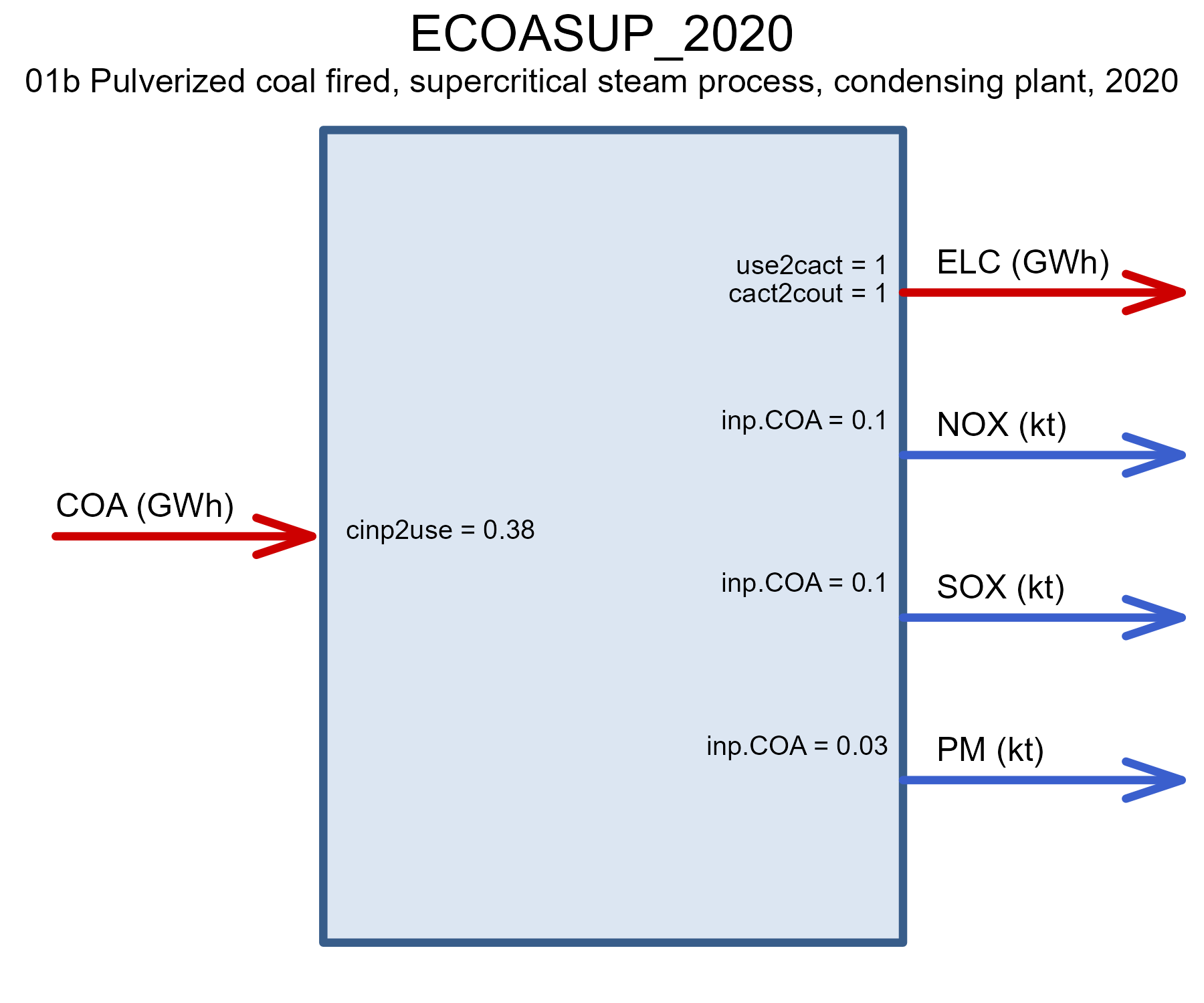

# draw(ECOA@data$ECOAULT_2050) # ultra-super-critical technology in 2050
# par(mfrow = par_init$mfrow) # reset to initial settings

Natural gas

There are two key natural gas fired technologies in the model: the combined cycle gas turbine (CCGT) and the open cycle gas turbine (OCGT). The existing capacity of gas-fired power plants in this example is assumed to be represented by the CCGT (ENGCC) technology, which will linearly retire by 2040. The OCGT technology (ENGOC) and more advanced vintages of NGCC are available for investment. The technology with carbon capture is defined the the CCS section below.

cap_gas <- cap |> # existing capacity
  filter(grepl("Gas", primary_fuel)) |>
  filter(!offshore) |>
  mutate(year = 2020, .before = 1)

# assume retirement of 2020 capacity by 2030
cap_gas_2030 <- cap_gas |>
  mutate(year = 2030, capacity_mw = 0.8 * capacity_mw)

# assume retirement of 2020 capacity by 2030
cap_gas_2040 <- cap_gas |>
  mutate(year = 2040, capacity_mw = 0.1 * capacity_mw)

# combine
cap_gas <- cap_gas |>
  bind_rows(cap_gas_2030) |>
  bind_rows(cap_gas_2040)
# Note: the existing capacity will be linearly interpolated from 2020 to 2040
# cap = 0 after 2040

# load coal technology (assume Super-critical for all existing capacity)
ENGCC_2020 <- ideea_modules$techs$ENGCC@data$ENGCC_2020

# update base-year technology with preexisting capacity
ENGCC_2020 <- ENGCC_2020 |>
  update(capacity = data.frame(
    region = cap_gas[[regN]],
    year = cap_gas$year,
    stock = cap_gas$capacity_mw / 1e3 # in GW
  ))

# load most advanced coal techs for new investment
EGAS <- ideea_modules$techs$ENGCC |> # Combined cycle gas turbine
  add(ENGCC_2020, overwrite = T) |> # technology with pre-existing capacity
  add(ideea_modules$techs$ENGOC) # open cycle gas turbine
names(EGAS@data)
#> [1] "ENGCC_2020" "ENGCC_2030" "ENGCC_2040" "ENGCC_2050" "ENGOC_2020"
#> [6] "ENGOC_2030" "ENGOC_2040" "ENGOC_2050"

draw(EGAS@data$ENGCC_2020)

# draw(EGAS@data$ENGCC_2050)

Solar

The solar technologies are defined for the base-year of the model with pre-existing capacity from WRI datasets; the new technologies available for investment are represented by several vintages of solar PV technologies up to 2050.

# solar capacity in ~2020
cap_sol_2020 <- cap |>
  filter(grepl("Solar", primary_fuel)) |>
  mutate(year = 2020, .before = 1)

cap_sol <- cap_sol_2020 # base year

# assume retirement of 2020 capacity by 2030
cap_sol_2030 <- cap_sol |>
  mutate(year = 2030, capacity_mw = 0.8 * capacity_mw)

# assume further retirement by 2040
cap_sol_2040 <- cap_sol |>
  mutate(year = 2040, capacity_mw = 0.1 * capacity_mw)

# combine
cap_sol <- cap_sol |>
  bind_rows(cap_sol_2030) |>
  bind_rows(cap_sol_2040)
# Note: the existing capacity will be linearly interpolated from 2020 to 2040
# cap = 0 after 2040

# Create two alternative repositories with solar technologies and constraints
# only one of the versions will be used in the model with equal results
# but both are created here for demonstration purposes
# version "const" is using explicit constraints on the capacity
ESOL_w_const <- newRepository(
  name = "solar_panels_w_const",
  desc = "Solar panels with cluster constraints on GW capacity")
# version "land" is using land resource as an auxiliary input
ESOL_w_land <- newRepository(
  name = "solar_panels_w_land",
  desc = "Solar panels with land limits per cluster")

# Solar technologies from IDEEA repository.
class(ideea_modules$techs$ESOL) # repository with solar techs
#> [1] "repository"
#> attr(,"package")
#> [1] "energyRt"
names(ideea_modules$techs$ESOL)
#> [1] "ESOL_2020" "ESOL_2030" "ESOL_2040" "ESOL_2050"

for (w in WSOL@data) { # CF by clusters
  # stop() # use for debug
  cl <- get_cluster(w@name)
  stopifnot(!is.na(cl)) # check

  # calculate the upper capacity constraint by cluster
  cluster_land <- ideea_sol_cl_sf |>
    st_drop_geometry() |>
    filter(!offshore) |>
    filter(cluster %in% as.integer(cl)) |>
    select(all_of(c(regN, "land_comm", "cluster", "area", "MW_max"))) |>
    group_by(across(all_of(c(regN, "land_comm", "cluster")))) |>
    summarise(
      area_km2 = round(as.numeric(sum(area, na.rm = T)), 1),
      GW_max = round(sum(MW_max, na.rm = T) / 1e3, 3),
      .groups = "drop"
    ) |>
    as.data.table()

  # check data consistency
  stopifnot(all(cluster_land[[regN]] %in% w@region))
  stopifnot(length(unique(cluster_land$land_comm)) == 1)

  # Declare land commodity
  land_comm <- newCommodity(
    name = unique(cluster_land$land_comm),
    desc = paste0("Land resource for solar cluster ", cl),
    unit = "km2",
    timeframe = "ANNUAL"
  )

  # Declare land resource by solar cluster and region
  land_res <- newSupply(
    name = paste0("RES_", land_comm@name),
    commodity = land_comm@name,
    desc = paste0("Land resource for solar cluster ", cl),
    unit = "km2",
    region = unique(cluster_land[[regN]]),
    availability = data.frame(
      region = cluster_land[[regN]],
      # year = NA_integer_,
      ava.up = cluster_land$area_km2
    )
  )

  # temporary lists to store technologies for every cluster and every vintage
  techs_cl_const <- list() # version "const"
  techs_cl_land <- list() # version "land"
  for (tec in ideea_modules$techs$ESOL@data) { # loop over vintages
    # stop() # use for debug

    # update prototype technology, "const" version
    tec_w <- update(
      tec,
      name = name_with_cluster(paste0(tec@name, "_CL"), cl),
      weather = list(
        weather = w@name,
        waf.fx = 1
      ),
      input = list(comm = "REN", unit = "GWh", combustion = 0)
    )
    
    # "land" version of the technology has land-commodity as an auxiliary input
    tec_w_land <- update(
      tec_w,
      aux = list(
        acomm = land_comm@name,
        unit = "km2"
      ),
      aeff = list(
        acomm = land_comm@name,
        cap2ainp = 1e3 / sol_onshore_max_MW_km2 # GW/km2
      )
    )
    
    # add technology to the temporary lists
    techs_cl_const[[tec_w@name]] <- tec_w; rm(tec, tec_w)
    techs_cl_land[[tec_w_land@name]] <- tec_w_land; rm(tec_w_land)
  }
  
  # 
  CT_ESOL_CL <- newConstraint(
    name = paste0("CT_ESOL_CL", cl),
    desc = "Constraint on total solar plants by cluster",
    eq = "<=",
    for.each = list(
      year = NA,
      region = w@region
    ),
    variable = list(
      variable = "vTechCap",
      for.sum = list(
        tech = names(techs_cl_const), # list all technologies for the cluster
        years = NULL
      )
    ),
    rhs = data.frame(
      year = as.numeric(NA),
      region = cluster_land[[regN]],
      rhs = cluster_land$GW
    ),
    defVal = Inf,
    interpolation = "back.inter.forth"
  )
  
  # version "const"
  ESOL_w_const <- add(ESOL_w_const, techs_cl_const, CT_ESOL_CL)
  # version "land"
  ESOL_w_land <- add(ESOL_w_land, techs_cl_land, land_comm, land_res)
  rm(land_comm, land_res, techs_cl_const, techs_cl_land, CT_ESOL_CL)
  
}
summary(ESOL_w_const); names(ESOL_w_const) |> head()
#> constraint technology 
#>          8         32
#> [1] "ESOL_2020_CL01" "ESOL_2030_CL01" "ESOL_2040_CL01" "ESOL_2050_CL01"
#> [5] "CT_ESOL_CL01"   "ESOL_2020_CL02"
draw(ESOL_w_const$ESOL_2020_CL01)

summary(ESOL_w_land); names(ESOL_w_land) |> head()
#>  commodity     supply technology 
#>          8          8         32
#> [1] "ESOL_2020_CL01"    "ESOL_2030_CL01"    "ESOL_2040_CL01"   
#> [4] "ESOL_2050_CL01"    "LAND_SOL_CL01"     "RES_LAND_SOL_CL01"
draw(ESOL_w_land$ESOL_2020_CL01)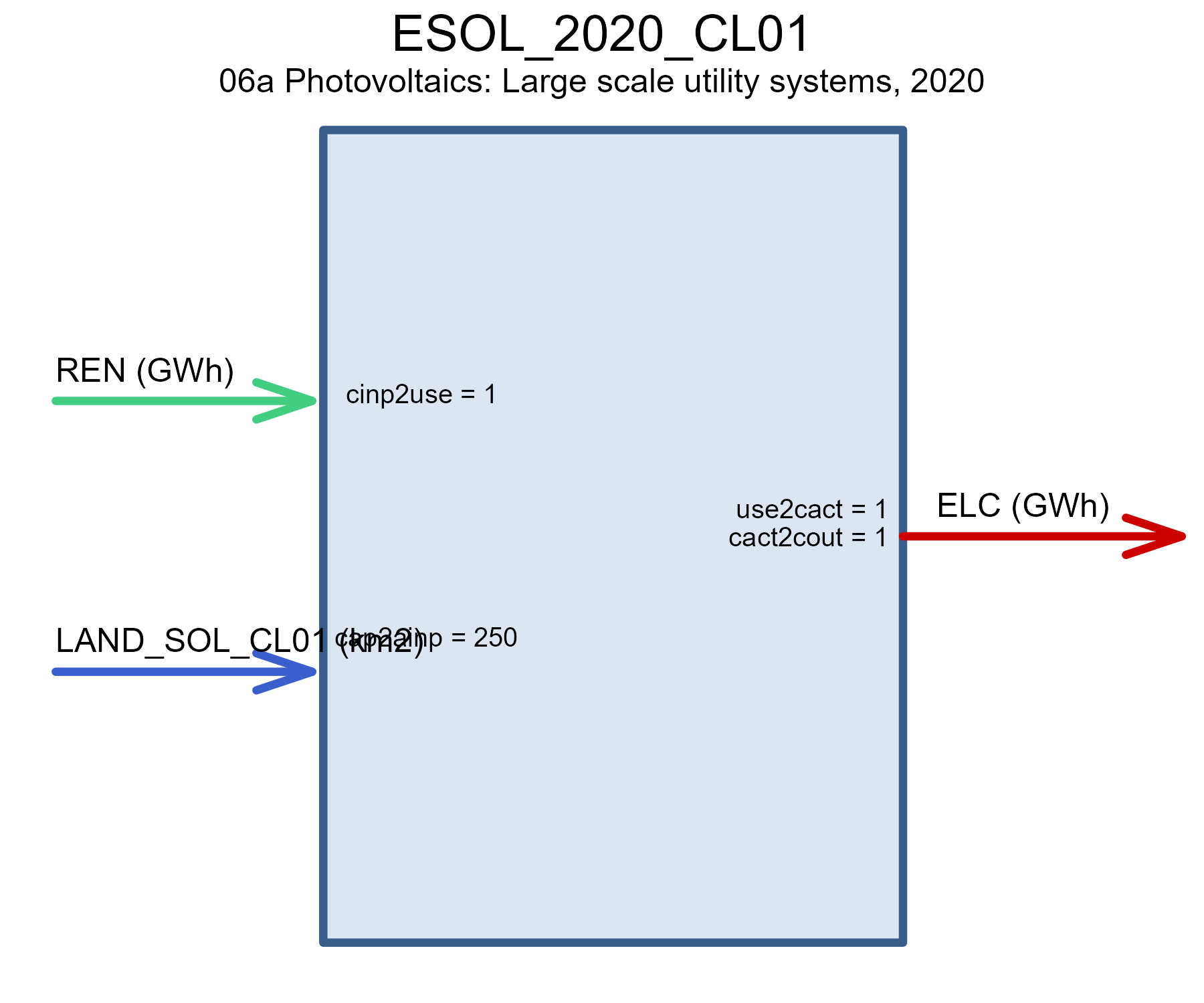

Wind

Similarly, the wind technologies are defined for the base-year of the model with pre-existing capacity from WRI datasets; the new technologies available for investment are represented by vintages.

Onshore

# existing capacity
cap_win <- cap |>
  filter(grepl("Wind", primary_fuel)) |>
  mutate(year = 2020, .before = 1)
# correcting the 2020 base year capacity values for wind.

# assume retirement of 2020 capacity by 2030
cap_win_2030 <- cap_win |>
  mutate(year = 2030, capacity_mw = 0.8 * capacity_mw)

# assume further retirement by 2040
cap_win_2040 <- cap_win |>
  mutate(year = 2040, capacity_mw = 0.1 * capacity_mw)

# combine
cap_win <- cap_win |>
  bind_rows(cap_win_2030) |>
  bind_rows(cap_win_2040)
# Note: the existing capacity will be linearly interpolated from 2020 to 2040
# cap = 0 after 2040

# Create two alternative repositories with wind technologies and constraints
# only one of the versions will be used in the model with equal results
# but both are created here for demonstration purposes
# version "const"
EWIN_w_const <- newRepository(
  name = "wind_turbines_const",
  desc = "Wind turbines with GW per cluster constraints")
# version "land"
EWIN_w_land <- newRepository(
  name = "wind_turbines_land",
  desc = "Wind turbines with land limits per cluster")

# Wind technologies from IDEEA repository
class(ideea_modules$techs$EWIN) # repository with wind techs
#> [1] "repository"
#> attr(,"package")
#> [1] "energyRt"
names(ideea_modules$techs$EWIN)
#> [1] "EWIN_2020" "EWIN_2030" "EWIN_2040" "EWIN_2050"

# Create technology for every cluster and every vintage
# (similar to solar above)
# wind_land_req <- ideea_win_cl_sf |>
#   st_drop_geometry() |>
#   select(all_of(c(regN, "offshore", "cluster", "area", "MW_max"))) |>
#   group_by(across(all_of(c(regN, "offshore", "cluster")))) |>
#   summarise(
#     area_km2 = round(as.numeric(sum(area, na.rm = T)), 1),
#     MW_max = sum(MW_max, na.rm = T), 
#     .groups = "drop") |>
#   as.data.table()

for (w in WWIN@data) { # CF by clusters
  # stop() # use for debug
  cl <- get_cluster(w@name)
  stopifnot(!is.na(cl)) # check

  # calculate the upper capacity constraint by cluster
  cluster_land <- ideea_win_cl_sf |>
    st_drop_geometry() |>
    filter(!offshore) |>
    filter(cluster %in% as.integer(cl)) |>
    select(all_of(c(regN, "land_comm", "cluster", "area", "MW_max"))) |>
    group_by(across(all_of(c(regN, "land_comm", "cluster")))) |>
    summarise(
      area_km2 = round(as.numeric(sum(area, na.rm = T)), 1),
      GW = round(sum(MW_max, na.rm = T) / 1e3, 3), 
      .groups = "drop"
      ) |>
    as.data.table()  
  
  # check data consistency
  stopifnot(all(cluster_land[[regN]] %in% w@region))
  stopifnot(length(unique(cluster_land$land_comm)) == 1)
  
  # Declare land commodity
  land_comm <- newCommodity(
    name = unique(cluster_land$land_comm),
    desc = paste0("Land resource for wind cluster ", cl),
    unit = "km2",
    timeframe = "ANNUAL"
  )
  
  # Declare land resource by wind cluster and region
  land_res <- newSupply(
    name = paste0("RES_", land_comm@name),
    commodity = land_comm@name,
    desc = paste0("Land resource for wind cluster ", cl),
    unit = "km2",
    region = unique(cluster_land[[regN]]),
    availability = data.frame(
      region = cluster_land[[regN]],
      # year = NA_integer_,
      ava.up = cluster_land$area_km2
    )
  )
  
  # temporary lists to store technologies for every cluster and every vintage
  techs_cl_const <- list() # version "const"
  techs_cl_land <- list() # version "land"
  for (tec in ideea_modules$techs$EWIN@data) { # loop over vintages
    # stop() # use for debug
    
    # update prototype technology, "const" version
    tec_w <- update(
      tec,
      name = name_with_cluster(paste0(tec@name, "_CL"), cl),
      weather = list(
        weather = w@name,
        waf.fx = 1
      ),
      input = list(comm = "REN", unit = "GWh", combustion = 0)
    )
    
    # "land" version of the technology has land-commodity as an auxiliary input
    tec_w_land <- update(
      tec_w,
      aux = list(
        acomm = land_comm@name,
        unit = "km2"
      ),
      aeff = list(
        acomm = land_comm@name,
        cap2ainp = 1e3 / win_onshore_max_MW_km2 # GW/km2
      )
    )

    # store in lists
    techs_cl_const[[tec_w@name]] <- tec_w; rm(tec, tec_w)
    techs_cl_land[[tec_w_land@name]] <- tec_w_land; rm(tec_w_land)
  }
  
  # assign base-year capacity to clusters 
  # (arbitrary, geo-location can be matched later)
  
  # stop()
  # make a capacity constraint for each cluster
  # cluster_GW_max <- ideea_win_cl_sf |>
  #   st_drop_geometry() |>
  #   # ungroup() |>
  #   filter(cluster %in% as.integer(cl)) |>
  #   filter(!offshore) |>
  #   select(all_of(c(regN, "cluster", "MW_max"))) |>
  #   group_by(across(c(regN, "cluster"))) |>
  #   summarise(GW = sum(MW_max, na.rm = T) / 1e3, .groups = "drop") |>
  #   as.data.table()
  
  # check data consistency
  # stopifnot(all(cluster_GW_max[[regN]] %in% w@region))
  
  # capacity constraint for version "const"
  CT_EWIN_CL <- newConstraint(
    name = paste0("CT_EWIN_CL", cl),
    desc = "Constraint on total solar plants by cluster",
    eq = "<=",
    for.each = list(
      year = NA, 
      region = w@region
    ),
    variable = list(
      variable = "vTechCap",
      for.sum = list(
        tech = names(techs_cl_const),
        years = NULL
      )
    ),
    rhs = data.frame(
      year = as.numeric(NA),
      region = cluster_land[[regN]],
      rhs = cluster_land$GW
    ),
    defVal = Inf,
    interpolation = "back.inter.forth"
  )
  # EWIN <- add(EWIN, lst_cl, CT_EWIN_CL); rm(lst_cl, CT_EWIN_CL)
  # EWIN <- add(EWIN, lst_cl); rm(lst_cl)
  
  # version "const"
  EWIN_w_const <- add(EWIN_w_const, techs_cl_const, CT_EWIN_CL)
  # version "land"
  EWIN_w_land <- add(EWIN_w_land, land_comm, land_res, techs_cl_land)
  rm(land_comm, land_res, techs_cl_const, techs_cl_land, CT_EWIN_CL)
}
summary(EWIN_w_const); names(EWIN_w_const) |> head()
#> constraint technology 
#>         12         48
#> [1] "EWIN_2020_CL01" "EWIN_2030_CL01" "EWIN_2040_CL01" "EWIN_2050_CL01"
#> [5] "CT_EWIN_CL01"   "EWIN_2020_CL02"
summary(EWIN_w_land); names(EWIN_w_land) |> head()
#>  commodity     supply technology 
#>         12         12         48
#> [1] "LAND_WIN_CL01"     "RES_LAND_WIN_CL01" "EWIN_2020_CL01"   
#> [4] "EWIN_2030_CL01"    "EWIN_2040_CL01"    "EWIN_2050_CL01"

# update base-year technology with preexisting capacity
# (assigning to first clusters, geo-location can be matched later)
# cap_win_exist <- cap_win |>
#   group_by(across(all_of(regN))) |>
#   summarise(GW_exist = max(capacity_mw) / 1e3, .groups = "drop") |>
#   rename(region = regN)
# 
# cap_win_exist_to_cluster <- EWIN$CT_EWIN_CL01@rhs |> 
#   right_join(cap_win_exist, by = "region") |>
#   filter(!is.na(rhs))
# 
# for (cl in 1:win_clust_max) {
#   
#   tname <- name_with_cluster("EWIN_2020_CL", cl, 
#                              ndigits = win_clust_digits)
#   cap_win_exist_to_cluster[[tname]] <-
#     cap_win_exist_to_cluster[["GW_exist"]]
#   
#   cap_win_exist_to_cluster[["diff"]] <-
#     cap_win_exist_to_cluster[["rhs"]] - cap_win_exist_to_cluster[[tname]]
#   
#   if (any(cap_win_exist_to_cluster[["diff"]] < 0)) {
#     ii <- cap_win_exist_to_cluster[["diff"]] >= 0
#     cap_win_exist_to_cluster[[tname]][!ii] <- 
#       cap_win_exist_to_cluster[["rhs"]][!ii]
#     cap_win_exist_to_cluster <-
#       cap_win_exist_to_cluster |>
#       mutate(
#         GW_exist = if_else(get("diff") >= 0, 0,
#                            -get("diff"))
#       )
#   } else {
#     cap_win_exist_to_cluster$GW_exist <- 0
#   }
#   capacity_cl = data.frame(
#       region = cap_win_exist_to_cluster$region,
#       year = cap_win_exist_to_cluster$year,
#       stock = cap_win_exist_to_cluster[[tname]] # in GW
#     ) |>
#     filter(stock > 0)
#   
#   EWIN@data[[tname]] <- EWIN@data[[tname]] |>
#     update(capacity = capacity_cl)
# 
#   if (any(cap_win_exist_to_cluster$GW_exist > 0)) break 
# }

# names(EWIN) |> head(); length(EWIN)
# EWIN@data$EWIN_2020_CL01@weather
# EWIN@data$EWIN_2020_CL01 |> draw()

Offshore

# (assuming) the existing capacity of offshore wind is zero

# Create a repository for offshore wind technologies
# "const" version
EWIF_w_const <- newRepository(
  name = "offshore_wind_turbines_const",
  desc = "Offshore wind turbines with GW per cluster constraints")
# "land" version
EWIF_w_land <- newRepository(
  name = "offshore_wind_turbines_land",
  desc = "Offshore wind turbines with land limits per cluster")

# Wind technologies from IDEEA repository
class(ideea_modules$techs$EWIF) # repository with wind techs
#> [1] "repository"
#> attr(,"package")
#> [1] "energyRt"
names(ideea_modules$techs$EWIF)
#> [1] "EWIF_2020" "EWIF_2030" "EWIF_2040" "EWIF_2050"

# Create technology for every cluster and every vintage
# (similar to solar above)
for (w in WWIF@data) { # CF by clusters
  # stop() # use for debug
  cl <- get_cluster(w@name)
  # land_comm <- paste0("LWIF_CL", cl)
  stopifnot(!is.na(cl))
  
  # calculate the upper capacity constraint by cluster
  cluster_land <- ideea_win_cl_sf |>
    st_drop_geometry() |>
    filter(offshore) |>
    filter(cluster %in% as.integer(cl)) |>
    select(all_of(c(regN, "land_comm", "cluster", "area", "MW_max"))) |>
    group_by(across(all_of(c(regN, "land_comm", "cluster")))) |>
    summarise(
      area_km2 = round(as.numeric(sum(area, na.rm = T)), 1),
      GW = round(sum(MW_max, na.rm = T) / 1e3, 1), 
      .groups = "drop") |>
    as.data.table()  
  
  # check data consistency
  stopifnot(all(cluster_land[[regN]] %in% w@region))
  stopifnot(length(unique(cluster_land$land_comm)) == 1)
  
  # Declare land commodity
  land_comm <- newCommodity(
    name = unique(cluster_land$land_comm),
    desc = paste0("Land (surface) for offshore wind cluster ", cl),
    unit = "km2",
    timeframe = "ANNUAL"
  )
  
  # Declare land resource by wind cluster and region
  land_res <- newSupply(
    name = paste0("RES_", land_comm@name),
    commodity = land_comm@name,
    desc = paste0("Land (surface) resource for offshore wind cluster ", cl),
    unit = "km2",
    region = unique(cluster_land[[regN]]),
    availability = data.frame(
      region = cluster_land[[regN]],
      # year = NA_integer_,
      ava.up = cluster_land$area_km2
    )
  )
  
  # lst_cl <- list() # temporary list
  techs_cl_const <- list() # version "const"
  techs_cl_land <- list() # version "land"
  for (tec in ideea_modules$techs$EWIF@data) { # vintages
    # stop() # use for debug
    # update prototype technology
    tec_w <- update(
      tec,
      name = name_with_cluster(paste0(tec@name, "_CL"), cl),
      weather = list(
        weather = w@name,
        waf.fx = 1
      ),
      input = list(comm = "REN", unit = "GWh", combustion = 0)
    )
    
    # "land" version of the technology has land-commodity as an auxiliary input
    tec_w_land <- update(
      tec_w,
      aux = list(
        acomm = land_comm@name,
        unit = "km2"
      ),
      aeff = list(
        acomm = land_comm@name,
        cap2ainp = 1e3 / win_offshore_max_MW_km2 # GW/km2
      )
    )
    
    # store in list
    # lst_cl[[tec_w@name]] <- tec_w; rm(tec, tec_w)
    techs_cl_const[[tec_w@name]] <- tec_w; rm(tec, tec_w)
    techs_cl_land[[tec_w_land@name]] <- tec_w_land; rm(tec_w_land)
  }
  # stop()
  # make a capacity constraint for each cluster
  # cluster_GW_max <- ideea_win_cl_sf |>
  #   st_drop_geometry() |>
  #   # ungroup() |>
  #   filter(cluster %in% as.integer(cl)) |>
  #   filter(offshore) |>
  #   select(all_of(c(regN, "cluster", "MW_max"))) |>
  #   group_by(across(c(regN, "cluster"))) |>
  #   summarise(GW = sum(MW_max, na.rm = T) / 1e3, .groups = "drop") |>
  #   as.data.table()
  # 
  # check data consistency
  # stopifnot(all(cluster_GW_max[[regN]] %in% w@region))
  
  # create capacity constraint
  CT_EWIF_CL <- newConstraint(
    name = paste0("CT_EWIF_CL", cl),
    # desc = "Constraint on total solar plants by cluster",
    eq = "<=",
    for.each = list(
      year = NA,
      region = w@region
    ),
    variable = list(
      variable = "vTechCap",
      for.sum = list(
        tech = names(techs_cl_const),
        years = NULL
      )
    ),
    rhs = data.frame(
      year = as.numeric(NA),
      region = cluster_land[[regN]],
      rhs = cluster_land$GW
    ),
    defVal = Inf,
    interpolation = "back.inter.forth"
  )
  # EWIF <- add(EWIF, lst_cl, CT_EWIF_CL); rm(lst_cl, CT_EWIF_CL)
  # EWIF <- add(EWIF, lst_cl); rm(lst_cl)
  # EWIF <- add(EWIF, land_comm, land_res, lst_cl)
  # rm(land_comm, land_res, lst_cl, cluster_land)
  EWIF_w_const <- add(EWIF_w_const, techs_cl_const, CT_EWIF_CL)
  EWIF_w_land <- add(EWIF_w_land, land_comm, land_res, techs_cl_land)
  rm(land_comm, land_res, techs_cl_const, techs_cl_land, CT_EWIF_CL)
}
summary(EWIF_w_const); names(EWIF_w_const) |> head()
#> constraint technology 
#>          7         28
#> [1] "EWIF_2020_CL01" "EWIF_2030_CL01" "EWIF_2040_CL01" "EWIF_2050_CL01"
#> [5] "CT_EWIF_CL01"   "EWIF_2020_CL02"
summary(EWIF_w_land); names(EWIF_w_land) |> head()
#>  commodity     supply technology 
#>          7          7         28
#> [1] "LAND_WIF_CL01"     "RES_LAND_WIF_CL01" "EWIF_2020_CL01"   
#> [4] "EWIF_2030_CL01"    "EWIF_2040_CL01"    "EWIF_2050_CL01"

Hydro

The decision on development of hydro-power plants normally goes beyond the optimization of costs, and takes into account the environmental and social impacts, as well as the availability of the water resources. The development of hydro-power may take a decade, and the operational lifetime can go beyond a century. Here we assume that the existing capacity of hydro-power plants do not retire (until 2100), the new investments are not available, such projects can be added to the model as a separate scenario.

cap_hyd <- cap |>
  filter(grepl("Hydro", primary_fuel)) |>
  mutate(primary_fuel = "Hydro") |> # combining Small with other - assumption (!)
  # filter(!offshore) |>
  group_by(across(any_of(
    c(regN, regN_off, "offshore", "primary_fuel")
  ))) |>
  summarise(capacity_mw = sum(capacity_mw, na.rm = T), .groups = "drop") |>
  filter(capacity_mw > 0) |>
  mutate(year = 2020, .before = 1)

# assume retirement of 2020 capacity by 2030
cap_hyd_2030 <- cap_hyd |>
  mutate(year = 2030, capacity_mw = 1 * capacity_mw)

# assume retirement of 2020 capacity by 2030
cap_hyd_2100 <- cap_hyd |>
  mutate(year = 2100, capacity_mw = 1 * capacity_mw)

# combine
cap_hyd <- cap_hyd |>
  bind_rows(cap_hyd_2030) |>
  bind_rows(cap_hyd_2100)
# Note: the existing capacity will be linearly interpolated from 2020 to 2040
# cap = 0 after 2040

# load base-year technology
EHYD_2020 <- ideea_modules$techs$EHYD@data$EHYD_2020
class(EHYD_2020)
#> [1] "technology"
#> attr(,"package")
#> [1] "energyRt"

# update base-year technology with preexisting capacity
EHYD_2020 <- EHYD_2020 |>
  update(
    capacity = data.frame(
      region = cap_hyd[[regN]],
      year = cap_hyd$year,
      stock = cap_hyd$capacity_mw / 1e3 # in GW
    ),
    end = list(end = 2010) # not available for investment
  )

EHYD <- ideea_modules$techs$EHYD |> #
  add(EHYD_2020, overwrite = T) # add tech with existing capacity
names(EHYD@data)
#> [1] "EHYD_2020" "EHYD_2030" "EHYD_2040" "EHYD_2050"

# add weather factor name and parameter for each technology
EHYD@data <- lapply(EHYD@data, function(tech) {
  update(
    tech,
    weather = data.frame(weather = "WHYD", waf.fx = 1),
    input = list(comm = "REN", combustion = 0)
  )
})
names(EHYD@data)
#> [1] "EHYD_2020" "EHYD_2030" "EHYD_2040" "EHYD_2050"
EHYD@data$EHYD_2020@weather
#>   weather comm wafc.lo wafc.up wafc.fx waf.lo waf.up waf.fx wafs.lo wafs.up
#> 1    WHYD <NA>      NA      NA      NA     NA     NA      1      NA      NA
#>   wafs.fx
#> 1      NA

draw(EHYD@data$EHYD_2020)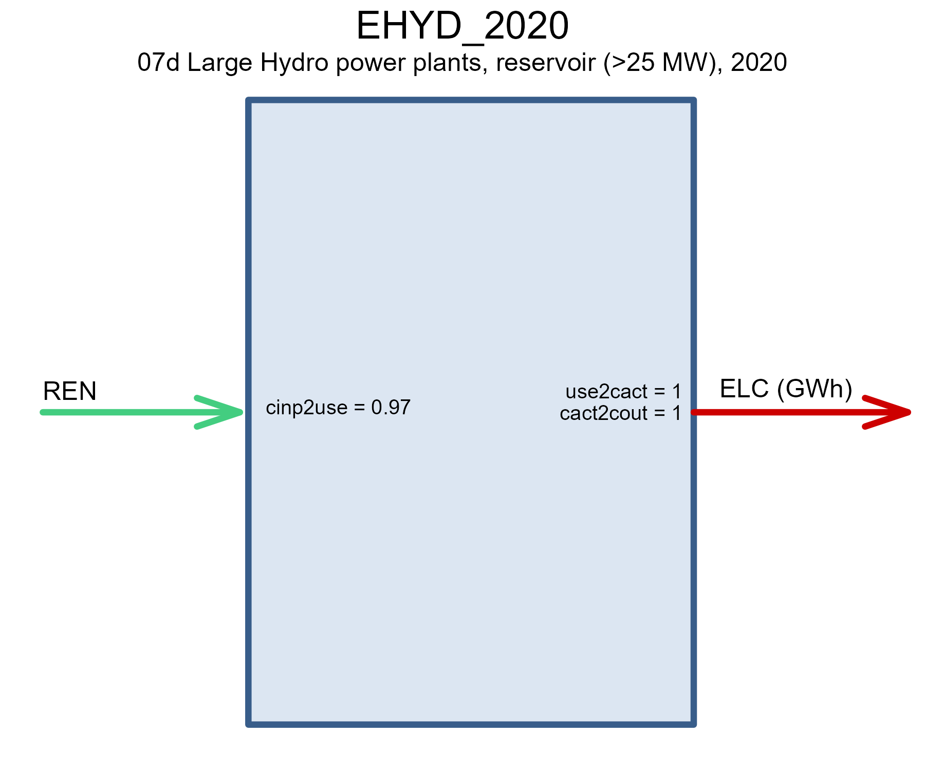

Nuclear

Nuclear power plants are also quite controversial, and the decision on their development is based on the long-term energy policy, the availability of the uranium resources, the safety and environmental concerns, and the public acceptance. Here we assume that the existing capacity of nuclear power plants do not retire (until 2050) with further linear fading out by 2080. The new investments are limited by a separate constraint (see Policies section), which can be dropped or relaxed in a particulate scenarios if decided.

cap_nuc <- cap |>
  filter(grepl("Nuclear", primary_fuel)) |>
  filter(!offshore) |>
  mutate(year = 2020, .before = 1)

# assume no retirement up to 2050
cap_nuc_2050 <- cap_nuc |>
  mutate(year = 2050, capacity_mw = 1 * capacity_mw)

# linear retirement from 2050 capacity by 2080
cap_nuc_LAST <- cap_nuc |>
  mutate(year = 2080, capacity_mw = 1e-20 * capacity_mw)

# combine
cap_nuc <- cap_nuc |>
  bind_rows(cap_nuc_2050) |>
  bind_rows(cap_nuc_LAST)

# load base-year technology
ENUC_2020 <- ideea_modules$techs$ENUC@data$ENUC_2020
class(ENUC_2020)
#> [1] "technology"
#> attr(,"package")
#> [1] "energyRt"

# update base-year technology with preexisting capacity
ENUC_2020 <- ENUC_2020 |>
  update(
    capacity = data.frame(
      region = cap_nuc[[regN]],
      year = cap_nuc$year,
      stock = cap_nuc$capacity_mw / 1e3 # in GW
    ),
    end = list(end = 2010) # not available for investment
  )

ENUC <- ideea_modules$techs$ENUC |> # all nuclear techs
  add(ENUC_2020, overwrite = T) # replace with the existing capacity
names(ENUC@data)
#> [1] "ENUC_2020" "ENUC_2030" "ENUC_2040" "ENUC_2050"

draw(ENUC@data$ENUC_2020)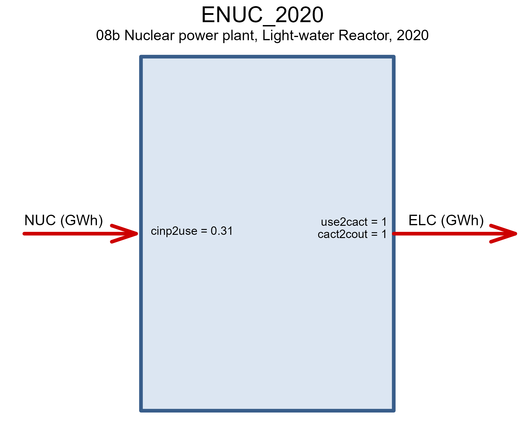

CCS

Coal- and gas-fired power plants with carbon capture and storage (CCS) technologies has been defined in “ccus” article and stored in the ideea_modules$CCUS repository. There are two types of CCS technologies: with fixed and flexible capture rates. The fixed capture rate is assumed to be used any time the technology produces electricity, while the flexible capture rate can be adjusted depending on the policy and carbon market conditions. Here we add the flexible CCS technologies.

# add coal and gas CCS techs from `ideea_modules$CCUS`
ccus_module <- ideea_modules$CCUS

repo_ccstechs <- newRepository(
  name = "CCS Technologies",
  desc = "Repository for CCS technologies",
  ccus_module$CCSCO2, # commodity to represent captured CO2
  ccus_module$GHG, # composite commodity--all GHGs
  
  ## option 1: Fixed CCS technology (see CCUS description)
  # ccus_module$ECOA_CCS_FX, # Coal plant with CCS
  # ccus_module$EGAS_CCS_FX, # Natural gas plant with CCS
  
  ## option 2: Variable CCS technology
  ccus_module$COA0, # coal commodity with captured CO2
  ccus_module$ALIAS_COA, # alias name COA == COA0 for supply
  ccus_module$ECOA_CCS_FL, # Coal power plant with variable CCS tech
  ccus_module$GAS0, # gas commodity with captured CO2
  ccus_module$ALIAS_GAS, # alias name GAS0 == CAS for supply
  ccus_module$EGAS_CCS_FL # gas power plant with variable CCS tech
)

rm(ccus_module)

Bio energy

The biomass-fired power plants are represented by the EBIO technology with the existing capacity from the WRI dataset. The new investments are available for the biomass technologies with different vintages up to 2050. We don’t consider CCS for biomass technologies in this example, but it can be added if needed.

cap_bio <- cap |>
  filter(grepl("Biomass", primary_fuel)) |>
  filter(!offshore) |>
  mutate(year = 2020, .before = 1)

# assume retirement of 2020 capacity by 2030
cap_bio_2030 <- cap_bio |>
  mutate(year = 2030, capacity_mw = 1 * capacity_mw)

# assume retirement of 2020 capacity by 2030
cap_bio_2060 <- cap_bio |>
  mutate(year = 2060, capacity_mw = 1 * capacity_mw)

# combine
cap_bio <- cap_bio |>
  bind_rows(cap_bio_2030) |>
  bind_rows(cap_bio_2060)

# load base-year technology
EBIO_2020 <- ideea_modules$techs$EBIO@data$EBIO_2020
class(EBIO_2020)
#> [1] "technology"
#> attr(,"package")
#> [1] "energyRt"

# update base-year technology with preexisting capacity
EBIO_2020 <- EBIO_2020 |>
  update(capacity = data.frame(
    region = cap_bio[[regN]],
    year = cap_bio$year,
    stock = cap_bio$capacity_mw / 1e3 # in GW
  ))

EBIO <- ideea_modules$techs$EBIO |> #
  add(EBIO_2020, overwrite = T) # add tech with existing capacity
names(EBIO@data)
#> [1] "EBIO_2020" "EBIO_2030" "EBIO_2040" "EBIO_2050"

draw(EBIO@data$EBIO_2020)

Energy storage

# ideea_modules$techs
STG_BTR <- ideea_modules$techs$STG_BTR
STG_BTR$STG_BTR_2020@fullYear # storage cycle over year or withing YDAY
#> [1] TRUE

# create daily storage (optional)
STG_BTR_daily <- STG_BTR
STG_BTR_daily@data <- lapply(STG_BTR_daily@data, function(ob) {
  if (.hasSlot(ob, "fullYear")) ob@fullYear <- FALSE
  ob
})
STG_BTR_daily$STG_BTR_2020@fullYear
#> [1] FALSE

Transmission

HVAC

HVAC cost: INR 1.56 Cr/km/GW Losses: 7%-10% per 1000km HVDC Cost: INR 3-5 Cr/km Losses: 1-3% per 1000km

network <- ideea_data$transmission[[regN]] |>
  filter(case == transmission_matrix, !is.na(MW)) |>
  # rename(dst = region1) |>
  filter(MW >= 0)

repo_transmission_ac <- newRepository("transmission")
if (nrow(network) > 0) {
  for (i in 1:nrow(network)) {
    trd <- newTrade(
      name = network$trd_name_ac[i],
      desc = paste0("Bi-directional HVAC transmission line between ",
                    network$region.x[i], " and ",
                    network$region.y[i], 
                    ifelse(is.null(network$lines_type[i]), "", 
                           paste0(" (", network$lines_type[i], ")"))
                    ),
      commodity = "ELC",
      routes = data.frame(
        src = c(network$region.x[i], network$region.y[i]),
        dst = c(network$region.y[i], network$region.x[i])
      ),
      trade = data.frame(
        src = c(network$region.x[i], network$region.y[i]),
        dst = c(network$region.y[i], network$region.x[i]),
        teff = c(network$AC_eff[i], network$AC_eff[i])
      ),
      capacityVariable = T,
      invcost = data.frame(
        # convert(1000, "USD/MW/mi", "cr.INR/GW/km") ~= 5 cr.INR/GW/km
        # see: https://www.nrel.gov/docs/fy22osti/81662.pdf
        region = c(network$region.x[i], network$region.y[i]),
        invcost = rep(network$AC_invcost[i] / 2, 2) # olife == 2
      ),
      olife = list(olife = 60), # doubled annualized invcost for consistency
      start = list(start = base_year - 10),
      capacity = data.frame(
        year = c(2020, 2030, 2050, 2070),
        stock = c(
          network$MW[i] / 1000, network$MW[i] / 1000,
          network$MW[i] / 1000, network$MW[i] / 1000
        ),
        # ncap.up = 5, # upper limit on new transmission by year
        cap.up = max(2 * network$MW[i] / 1000 + 10, 10) # upper limit on transmission capacity
      ),
      cap2act = 24 * 365
    )
    repo_transmission_ac <- add(repo_transmission_ac, trd)
    rm(trd)
  }
}
names(repo_transmission_ac)
#>  [1] "HVAC_APY_OR"  "HVAC_APY_TG"  "HVAC_APY_TNY" "HVAC_AR_AS"   "HVAC_AR_NL"  
#>  [6] "HVAC_AS_ML"   "HVAC_BR_CT"   "HVAC_BR_JH"   "HVAC_BR_SK"   "HVAC_BR_UP"  
#> [11] "HVAC_CT_MP"   "HVAC_CT_OR"   "HVAC_CT_TG"   "HVAC_DL_HR"   "HVAC_DL_RJ"  
#> [16] "HVAC_DL_UP"   "HVAC_DL_UT"   "HVAC_GA_GJN"  "HVAC_GA_KA"   "HVAC_GA_KLY" 
#> [21] "HVAC_GA_MH"   "HVAC_GJN_MH"  "HVAC_GJN_MP"  "HVAC_GJN_RJ"  "HVAC_HP_JK"  
#> [26] "HVAC_HP_PBH"  "HVAC_HP_UT"   "HVAC_HR_PBH"  "HVAC_JH_OR"   "HVAC_JH_WB"  
#> [31] "HVAC_KA_KLY"  "HVAC_KA_TG"   "HVAC_KA_TNY"  "HVAC_KLY_TNY" "HVAC_MH_MP"  
#> [36] "HVAC_MH_TG"   "HVAC_ML_SK"   "HVAC_ML_TR"   "HVAC_MN_MZ"   "HVAC_MN_NL"  
#> [41] "HVAC_MP_RJ"   "HVAC_MP_UP"   "HVAC_MZ_TR"   "HVAC_OR_WB"   "HVAC_PBH_RJ" 
#> [46] "HVAC_SK_WB"   "HVAC_TR_WB"   "HVAC_UP_UT"
repo_transmission_ac[[1]]
#> An object of class "trade"
#> Slot "name":
#> [1] "HVAC_APY_OR"
#> 
#> Slot "desc":
#> [1] "Bi-directional HVAC transmission line between APY and OR"
#> 
#> Slot "commodity":
#> [1] "ELC"
#> 
#> Slot "routes":
#>   src dst
#> 1 APY  OR
#> 2  OR APY
#> 
#> Slot "trade":
#>   src dst year slice ava.up ava.fx ava.lo      teff
#> 1 APY  OR   NA  <NA>     NA     NA     NA 0.9244707
#> 2  OR APY   NA  <NA>     NA     NA     NA 0.9244707
#> 
#> Slot "aux":
#> [1] acomm unit 
#> <0 rows> (or 0-length row.names)
#> 
#> Slot "aeff":
#> [1] acomm     src       dst       year      slice     csrc2aout csrc2ainp
#> [8] cdst2aout cdst2ainp
#> <0 rows> (or 0-length row.names)
#> 
#> Slot "invcost":
#>   region year invcost wacc retcost
#> 1    APY   NA     817   NA      NA
#> 2     OR   NA     817   NA      NA
#> 
#> Slot "fixom":
#> [1] region year   fixom 
#> <0 rows> (or 0-length row.names)
#> 
#> Slot "varom":
#> [1] src    dst    year   varom  markup
#> <0 rows> (or 0-length row.names)
#> 
#> Slot "olife":
#>   year olife
#> 1   NA    60
#> 
#> Slot "start":
#>   start
#> 1  2009
#> 
#> Slot "end":
#>   end
#> 1 Inf
#> 
#> Slot "capacity":
#>   year stock cap.lo cap.up cap.fx ncap.lo ncap.up ncap.fx ret.lo ret.up ret.fx
#> 1 2020     0     NA     10     NA      NA      NA      NA     NA     NA     NA
#> 2 2030     0     NA     10     NA      NA      NA      NA     NA     NA     NA
#> 3 2050     0     NA     10     NA      NA      NA      NA     NA     NA     NA
#> 4 2070     0     NA     10     NA      NA      NA      NA     NA     NA     NA
#> 
#> Slot "capacityVariable":
#> [1] TRUE
#> 
#> Slot "cap2act":
#> [1] 8760
#> 
#> Slot "optimizeRetirement":
#> [1] FALSE
#> 
#> Slot "misc":
#> list()

HVDC

EDC <- newCommodity(
  name = "EDC",
  desc = "Ultra high voltage DC electricity",
  unit = "GWh"
)

# Converters (inverter and rectifier stations)
EDC2ELC <- newTechnology(
  name = "EDC2ELC",
  desc = "Inverter station",
  input = list(comm = "EDC", unit = "GWh"),
  output = list(comm = "ELC", unit = "GWh"),
  invcost = list(
    invcost = 500
  ), 
  ceff = list(
    comm = "ELC",
    cact2cout = .99
    ),
  olife = list(olife = 30),
  cap2act = 24 * 365
)
draw(EDC2ELC)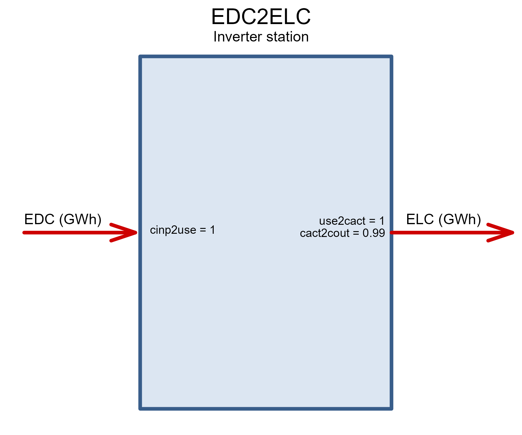

ELC2EDC <- newTechnology(
  name = "ELC2EDC",
  desc = "Rectifier station",
  output = list(comm = "EDC", unit = "GWh"),
  input = list(comm = "ELC", unit = "GWh"),
  invcost = list(
    invcost = 500
  ), 
  ceff = list(
    comm = "EDC",
    cact2cout = .99),
  olife = list(olife = 30),
  cap2act = 24 * 365
)
draw(ELC2EDC)

repo_transmission_dc <- 
  newRepository(name = "transmission_dc", EDC, EDC2ELC, ELC2EDC)

if (nrow(network) > 0) {
  for (i in 1:nrow(network)) {
    trd <- newTrade(
      name = network$trd_name_dc[i],
      desc = paste0("Bi-directional HVDC transmission line between ",
                    network$region.x[i], " and ",
                    network$region.y[i], 
                    ifelse(is.null(network$lines_type[i]), "", 
                           paste0(" (", network$lines_type[i], ")"))
                    ),
      commodity = "EDC",
      routes = data.frame(
        src = c(network$region.x[i], network$region.y[i]),
        dst = c(network$region.y[i], network$region.x[i])
      ),
      trade = data.frame(
        src = c(network$region.x[i], network$region.y[i]),
        dst = c(network$region.y[i], network$region.x[i]),
        teff = c(network$DC_eff[i], network$DC_eff[i])
      ),
      capacityVariable = T,
      invcost = data.frame(
        # convert(1000, "USD/MW/mi", "cr.INR/GW/km") ~= 5 cr.INR/GW/km
        # see: https://www.nrel.gov/docs/fy22osti/81662.pdf
        region = c(network$region.x[i], network$region.y[i]),
        invcost = rep(network$DC_invcost[i] / 2, 2) # olife == 2
      ),
      olife = list(olife = 60), # doubled annualized invcost for consistency
      start = list(start = base_year - 10),
      capacity = data.frame(
        year = c(2020, 2030, 2050, 2070),
        stock = c(
          network$MW[i] / 1000, network$MW[i] / 1000,
          network$MW[i] / 1000, network$MW[i] / 1000
        ),
        cap.up = 100 # upper limit on transmission capacity
      ),
      cap2act = 24 * 365
    )
    repo_transmission_dc <- add(repo_transmission_dc, trd)
    rm(trd)
  }
}
names(repo_transmission_dc)
#>  [1] "EDC"          "EDC2ELC"      "ELC2EDC"      "HVDC_APY_OR"  "HVDC_APY_TG" 
#>  [6] "HVDC_APY_TNY" "HVDC_AR_AS"   "HVDC_AR_NL"   "HVDC_AS_ML"   "HVDC_BR_CT"  
#> [11] "HVDC_BR_JH"   "HVDC_BR_SK"   "HVDC_BR_UP"   "HVDC_CT_MP"   "HVDC_CT_OR"  
#> [16] "HVDC_CT_TG"   "HVDC_DL_HR"   "HVDC_DL_RJ"   "HVDC_DL_UP"   "HVDC_DL_UT"  
#> [21] "HVDC_GA_GJN"  "HVDC_GA_KA"   "HVDC_GA_KLY"  "HVDC_GA_MH"   "HVDC_GJN_MH" 
#> [26] "HVDC_GJN_MP"  "HVDC_GJN_RJ"  "HVDC_HP_JK"   "HVDC_HP_PBH"  "HVDC_HP_UT"  
#> [31] "HVDC_HR_PBH"  "HVDC_JH_OR"   "HVDC_JH_WB"   "HVDC_KA_KLY"  "HVDC_KA_TG"  
#> [36] "HVDC_KA_TNY"  "HVDC_KLY_TNY" "HVDC_MH_MP"   "HVDC_MH_TG"   "HVDC_ML_SK"  
#> [41] "HVDC_ML_TR"   "HVDC_MN_MZ"   "HVDC_MN_NL"   "HVDC_MP_RJ"   "HVDC_MP_UP"  
#> [46] "HVDC_MZ_TR"   "HVDC_OR_WB"   "HVDC_PBH_RJ"  "HVDC_SK_WB"   "HVDC_TR_WB"  
#> [51] "HVDC_UP_UT"
# (optional) filter out some lines in mountainous regions
repo_transmission_dc@data[["HVDC_HP_JK"]] <- NULL
repo_transmission_dc@data[["HVDC_SK_WB"]] <- NULL
repo_transmission_dc@data[["HVDC_BR_SK"]] <- NULL
repo_transmission_dc@data[["HVDC_ML_SK"]] <- NULL

Unserved load

UNSERVED <- newImport(
  name = "UNSERVED",
  desc = "Unserved load, ~ 10 cr.INR/GWh, equal 100 INR/kWh",
  commodity = "ELC",
  unit = "GWh",
  imp = list(price = 100)
)

Policies

carbon emissions, climate, air quality, SOx, NOx, PM, etc.
* national
* state, local
any other regulations of electric power sector

CO2_CAP <- newConstraint(
  name = "CO2_CAP",
  eq = "<=",
  rhs = list(
    year = c(2025, 2060, 2100),
    rhs = c(900000, 1e-10, 1e-10) # CO2 cap assumptions
  ),
  for.each = list(year = 2025:2100), # Cap total emission
  variable = list(
    variable = "vBalance",
    for.sum = list(
      comm = "CO2",
      slice = NULL,
      region = NULL
    )
  ),
  defVal = Inf,
  interpolation = "inter.forth"
)
CO2_CAP@rhs
#>   year   rhs
#> 1 2025 9e+05
#> 2 2060 1e-10
#> 3 2100 1e-10

NO_NEW_HYDRO <- newConstraint(
  name = "NO_NEW_HYDRO",
  # desc = "Constraint on new Hydro plants construction",
  eq = "<=",
  for.each = list(year = NULL),
  variable = list(
    variable = "vTechNewCap",
    for.sum = list(
      tech = c("EHYD_2030", "EHYD_2040", "EHYD_2050", "EHYD_2020"),
      region = NULL
    )
  ),
  rhs = data.frame(
    year = c(2020, 2060),
    rhs = c(1e-20)
  ),
  defVal = 1e-20,
  interpolation = "inter.forth"
)

NO_NEW_NUCLEAR <- newConstraint(
  name = "NO_NEW_NUCLEAR",
  # desc = "Constraint on new Hydro plants construction",
  eq = "<=",
  for.each = list(year = 2020:2060),
  variable = list(
    variable = "vTechNewCap",
    for.sum = list(
      tech = c("ENUC_2030", "ENUC_2040", "ENUC_2050", "ENUC_2020"),
      region = NULL
    )
  ),
  rhs = data.frame(
    year = c(2020:2060),
    rhs = 1e-20
    # rhs = c(1e-7) #eps
  ),
  defVal = 1e-20,
  interpolation = "inter.forth"
)

# dput(names(ESOL))
NO_NEW_SOLAR <- newConstraint(
  name = "NO_NEW_SOLAR",
  # desc = "Constraint on new Hydro plants construction",
  eq = "<=",
  for.each = list(year = 2020:2060),
  variable = list(
    variable = "vTechNewCap",
    for.sum = list(
      tech = names(ESOL_w_const)[grepl("^ESOL", names(ESOL_w_const))],
      region = NULL
    )
  ),
  rhs = data.frame(
    year = c(2020:2060),
    rhs = 1e-20
    # rhs = c(1e-7) #eps
  ),
  defVal = 1e-20,
  interpolation = "inter.forth"
)

NO_NEW_WIND <- newConstraint(
  name = "NO_NEW_WIND",
  # desc = "Constraint on new Hydro plants construction",
  eq = "<=",
  for.each = list(year = 2020:2060),
  variable = list(
    variable = "vTechNewCap",
    for.sum = list(
      tech = names(EWIN_w_const)[grepl("^EWIN", names(EWIN_w_const))],
      region = NULL
    )
  ),
  rhs = data.frame(
    year = c(2020:2060),
    rhs = 1e-20
  ),
  defVal = 1e-20,
  interpolation = "inter.forth"
)

# dput(names(EGAS))
CT_EGAS <- newConstraint(
  name = "CT_EGAS",
  # desc = "Constraint on new Hydro plants construction",
  eq = "<=",
  for.each = list(year = c(2020, 2055)),
  variable = list(
    variable = "vTechNewCap",
    for.sum = list(
      tech = names(EGAS),
      region = NULL
    )
  ),
  rhs = list(
    year = c(2020, 2055),
    rhs = c(5, 5)
  ),
  defVal = 1e-20,
  interpolation = "inter.forth"
)
# limit on hydro construction

# No Base year investment
NO_BY_INV <- newConstraint(
  name = "NO_BY_INV",
  eq = "<=",
  for.each = list(year = c(2020, 2021, 2060)),
  variable = list(
    variable = "vTechNewCap",
    for.sum = list(
      tech = NA,
      region = NA
    )
  ),
  rhs = data.frame(
    year = c(2020, 2021, 2060),
    rhs = c(1e-20, 1e10, 1e10) #
  ),
  defVal = 1e10, # large number (Inf may not work as expected in some solvers)
  interpolation = "inter.forth"
)

An optional, additional constraint on Solar Capacity Deployment across regions. By default, the constraint on capacity is set for every cluster of regions based on available (estimated) land area and solar radiation. However, the constraint can be adjusted for each region separately as defined below for 5-region model case.

if (nreg == 5) {
  # optional constraint for total solar capacity on top of cluster constraints
  CT_ESOL_TOT <- newConstraint(
    name = "CT_ESOL",
    desc = "Constraint on solar plants capacity by region",
    eq = "<=",
    for.each = list(
      year = NA,
      region = c("EAST", "NORTH", "NORTHEAST", "SOUTH", "WEST")
    ),
    variable = list(
      variable = "vTechCap",
      for.sum = list(
        # list all solar technologies
        tech = names(ESOL_w_const)[grepl("^ESOL", names(ESOL_w_const))],
        year = NULL
      )
    ),
    rhs = data.frame(
      year = as.numeric(NA),
      region = c("NORTH", "SOUTH", "EAST", "WEST", "NORTHEAST"),
      # adjust numbers according to your assumptions
      rhs = c(336.250, 107.330, 66.360, 180.9, 57.36) # upper limit
    ),
    defVal = Inf,
    interpolation = "back.inter.forth"
  )
} else { # for other models
  CT_ESOL_TOT <- NULL # adjust the above constraint for your model if needed
}

Model

repo <- newRepository(
  name = glue("repo_electricity_{regN}"),
  # commodities
  repo_comm,
  # supply & import
  repo_supply,
  # Generating technologies
  ECOA,
  EGAS, CT_EGAS, # gas-fired generators with limit on construction
  ENUC,
  NO_NEW_NUCLEAR, # limit on nuclear construction
  EHYD, WHYD,
  NO_NEW_HYDRO, # limit on hydro construction
  WSOL, # solar capacity factors
  ESOL_w_const, # solar generators with capacity constraints version
  # ESOL_w_land, # solar generators with land constraints version
  WWIN, # onshore wind capacity factors
  EWIN_w_const, # onshore wind generators with capacity constraints version
  # EWIN_w_land, # onshore wind generators with land constraints version
  WWIF, # offshore wind capacity factors
  EWIF_w_const, # offshore wind generators with capacity constraints version
  # EWIF_w_land, # offshore wind generators with land constraints version
  EBIO, 
  # battery
  STG_BTR, # storage with annual cycle
  # STG_BTR_daily, # alternative storage with daily cycle
  # transmission
  repo_transmission_ac,
  repo_transmission_dc,
  repo_geoccs,
  repo_ccstechs,
  # unserved load
  UNSERVED, # unserved load penalty
  # demand
  DEMELC_BY, # BY demand
  DEMELC_2X, # additional demand
  # CT_ESOL, # solar capacity constraints
  NO_BY_INV #
)

# print(repo)
# names(repo)
summary(repo)
#>  commodity constraint     demand     import    storage     supply technology 
#>         17         31          2          5          4          6        139 
#>      trade    weather 
#>         92         28

# model horizon
# horizon_2020_2060_by_10 <- newHorizon(
#   period = 2020:2060,
#   intervals = c(1, 5, rep(10, 15)),
#   mid_is_end = T
# )
# horizon_2020_2060_by_10

# model-class object
mod <- newModel(
  name = glue("IDEEA_ELC_{regN}"),
  desc = "IDEEA electricity example model",
  region = unique(ideea_sf[[regN]]),
  discount = 0.05,
  calendar = ideea_modules$calendars$calendar_d365_h24,
  horizon = ideea_modules$calendars$horizon_2020_2060_by_10,
  data = repo
)
# mod@config@horizon@intervals
# mod@config@calendar@timetable

Solving the model

Note: The full model requires powerful solver (CPLEX or GUROBI) and GAMS Julia or Python + CPLEX/GUROBI will also work, but currently require more time to generate the problem for the solver.
It is recommended to solve the model for a portion of a year (subset of time-slices), which can be solved with free solvers such as HiGHS or Cbc.

Reference scenario - subset

Quick way to have a glimpse of the results

# set_progress_bar("progress")
# Reference case
scen_REF_sub <- interpolate_model(
  mod,
  name = "REF_sub", # indicating 'subset'
  calendar = ideea_modules$calendars$calendar_d365_h24_subset_1day_per_month,
  horizon = ideea_modules$horizons$horizon_2050
)

# directory to store the scenario
scen_REF_sub@path 

scen_REF_sub <- write_sc(
  scen_REF_sub,
  solver = solver_options$gams_gdx_cplex_barrier
  # solver = solver_options$gams_gdx_cplex_parallel
  # solver = solver_options$julia_highs_barrier
  # solver = solver_options$julia_highs_simplex
  # solver = solver_options$julia_highs_parallel
)
scen_REF_sub@status
scen_REF_sub@misc$tmp.dir

# solve_scenario(scen_REF_sub, wait = F, force = F)
scen_REF_sub <- solve(scen_REF_sub, wait = F, tmp.del = F)
scen_REF_sub <- read(scen_REF_sub)

# store scenario on disk (unload from RAM)
scen_REF_sub <- save_scenario(scen_REF_sub)
summary(scen_REF_sub)

Policy scenarios

# CO2 cap
scen_CAP_sub <- interpolate(
  mod,
  name = "CAP_sub", # indicating 'subset'
  # path = file.path("scenarios", glue("CAP_sub_r{nreg}_debug")),
  # here we can add policy objects
  # STG_BTR_daily, # Battery, modeled with daily cycle for sampled calendar
  CO2_CAP,
  calendar = ideea_modules$calendars$calendar_d365_h24_subset_1day_per_month,
  # horizon = ideea_modules$calendars$horizon_2020_2060_by_10
  ideea_modules$horizons$horizon_2050
  # partial_calendar # add partial calendar to the interpolate function
)

# scen_CAP_sub@path <- file.path(
#   ideea_scenarios(),
#   ideea_scenario_dir_name(
#     name = "CAP_sub", 
#     model_name = mod@name, 
#     calendar_name = "d365_h24", 
#     horizon_name = "2050"
# ))
scen_CAP_sub@path

scen_CAP_sub <- write_sc(
  scen_CAP_sub,
  # solver = solver_options$gams_gdx_cplex_barrier
  # solver = solver_options$gams_gdx_cplex_parallel
  # solver = solver_options$pyomo_glpk
  # solver = solver_options$pyomo_cbc
  solver = solver_options$julia_highs_barrier
  # solver = solver_options$julia_highs_simplex
  # solver = solver_options$julia_highs_parallel
)
scen_CAP_sub
scen_CAP_sub@misc$tmp.dir

solve_scenario(scen_CAP_sub, wait = F, force = F)
# scen_CAP_sub <- solve(scen_CAP_sub, wait = T, tmp.del = F)
scen_CAP_sub <- read(scen_CAP_sub)

# store scenario on disk (unload from RAM)
scen_CAP_sub <- save_scenario(scen_CAP_sub)
summary(scen_CAP_sub)

scen_REF <- interpolate_model(
  mod, 
  name = "REF", 
  ideea_modules$horizons$horizon_2050
)
scen_REF

scen_REF <- write_sc(
  scen_REF,
  solver = solver_options$gams_gdx_cplex_barrier
  # solver = solver_options$gams_gdx_cplex_parallel
  # solver = solver_options$julia_highs_barrier
  # solver = solver_options$julia_highs_simplex
  # solver = solver_options$julia_highs_parallel
)
scen_REF@status
scen_REF@misc$tmp.dir

# solve_scenario(scen_REF, wait = F, force = F)
scen_REF <- solve(scen_REF, wait = F, tmp.del = F)
scen_REF <- read(scen_REF)

# store scenario on disk (unload from RAM)
scen_REF <- save_scenario(scen_REF)
summary(scen_REF)

set_progress_bar()

horizon_2040_2060_by_20 <-
  newHorizon(
    name = "hz2040-2060by20L1",
    period = 2040:2060,
    intervals = c(1, rep(20, 3)),
    # intervals = rep(20, 4), 
    mid_is_end = T
  )
horizon_2040_2060_by_20@intervals$start <- 
  horizon_2040_2060_by_20@intervals$end

# CO2 cap
scen_CAP <- interpolate(
  mod,
  name = "CAP", # indicating 'subset'
  # path = file.path("scenarios", glue("CAP_r{nreg}_debug")),
  # here we can add policy objects
  # STG_BTR_daily, # Battery, modeled with daily cycle for sampled calendar
  CO2_CAP,
  horizon_2040_2060_by_20
  # ideea_modules$horizons$horizon_2050
  # horizon_2050
  # partial_calendar # add partial calendar to the interpolate function
)

# scen_CAP@path <- file.path(
#   ideea_scenarios(),
#   ideea_scenario_dir_name(
#     name = "CAP", 
#     model_name = mod@name, 
#     calendar_name = "d365_h24", 
#     horizon_name = "2060"
#   ))
scen_CAP@path

scen_CAP <- write_sc(
  scen_CAP,
  solver = solver_options$gams_gdx_cplex_barrier
  # solver = solver_options$gams_gdx_cplex_parallel
  # solver = solver_options$pyomo_glpk
  # solver = solver_options$julia_highs_barrier
  # solver = solver_options$julia_highs_simplex
  # solver = solver_options$julia_highs_parallel
)
scen_CAP

# save(scen_CAP, file = file.path(scen_CAP@path, "scen_CAP_interpolated.RData"))

solve_scenario(scen_CAP, wait = F, force = F)
scen_CAP <- read(scen_CAP)
# scen_CAP <- solve(scen_CAP, wait = T, tmp.del = F)

# store scenario on disk (unload from RAM)
scen_CAP <- save_scenario(scen_CAP)
summary(scen_CAP)
# installr::os.sleep()

Results

Compare scenarios

# create a list of
sns <- list(
  # scen_REF,
  scen_CAP
  # scen_REF_sub
  # scen_CAP_sub
  # .scen$CAP_sub,
  # .scen$REF_sub
)

# compare objective (in cr.₹)
getData(sns, "vObjective", merge = T)
# use `?getData` for help

getData(sns, "vBalance", comm = "CO2", merge = T, digits = 1, 
        drop.zeros = T) |> 
  # group_by(name, year) |> 
  # summarize(GWh = sum(value)) |> 
  pivot_wider(names_from = scenario, values_from = value)

Total installed capacity

# compare generating tech capacity (names start with "E")
vTechCap <- getData(sns,
  name = "vTechCap", tech_ = "^E", process = T,
  merge = T, digits = 3, drop.zeros = T
)

vTechCap |>
  pivot_wider(names_from = scenario) |>
  as.data.table()

# getData(scen_CAP_sub, "vImportRow", imp = "UNSERVED",
#         digits = 1, drop.zeros = T, merge = T) |> 
#   group_by(name, comm) |> 
#   summarize(GWh = sum(value))

getData(sns, "pDemand", digits = 1, drop.zeros = T, merge = T) |> 
  group_by(scenario, name, comm) |> 
  summarize(GWh = sum(value))

Total capacity map

vTechCap_agg <- vTechCap |>
  drop_process_cluster() |>
  drop_process_vintage() |> 
  group_by(scenario, process, region, year) |>
  summarise(GW = sum(value, na.rm = T), .groups = "drop") |>
  as.data.table() |>
  full_join(ideea_sf, by = c(region = regN_off),
    relationship = "many-to-many") |>
  filter(!is.na(process)) |>
  # filter(year %in% c(2020, 2035, 2060)) |>
  st_as_sf()

ggplot() +
  geom_sf(data = ideea_sf) +
  geom_sf(aes(fill = GW), data = vTechCap_agg, na.rm = T) +
  scale_fill_viridis_c(option = "H", transform = "sqrt") +
  # scale_fill_viridis_c(option = "C", transform = "log10") +
  # facet_grid(process~scenario) +
  facet_wrap(scenario~process) +
  theme_ideea_map()

vTechCap_agg |> st_drop_geometry() |> 
  group_by(scenario, process, year) |>
  summarise(GW = sum(GW)) |>
  pivot_wider(names_from = scenario, values_from = GW)

Solar capacity by cluster

add_cluster_column <- function(x, col_name = "process") {
  x |> mutate(
    cluster = as.integer(str_extract(get(col_name), "[0-9]+$")),
    .after = col_name
  )
}

vTechCap_ESOL_sf <-
  vTechCap |>
  filter(grepl("ESOL", process)) |> # select solar techs
  add_cluster_column() |> # add cluster number
  # add shapes for every cluster
  left_join(ideea_sol_cl_sf,
    by = c(region = regN_off, cluster = "cluster"),
    relationship = "many-to-many"
  ) |>
  rename(GW = value) |>
  filter(!is.na(GW), GW > 0) |>
  # filter(year %in% c(2020, 2035, 2060)) |>
  st_as_sf() # force to treat 'geometry' column as shape-data

ggplot() +
  geom_sf(data = ideea_sf) +
  geom_sf(aes(fill = GW), data = vTechCap_ESOL_sf, color = NA, na.rm = T) +
  # scale_fill_viridis_c(option = "H") +
  scale_fill_viridis_c(option = "C", transform = "log10") +
  facet_grid(year ~ scenario) +
  theme_ideea_map()

Wind capacity by cluster

vTechCap_EWIN_sf <-
  vTechCap |>
  filter(grepl("EWIN", process)) |> # select solar techs
  add_cluster_column() |> # add cluster number
  # add shapes for every cluster
  left_join(ideea_win_cl_sf,
    by = c(region = regN_off, cluster = "cluster"),
    relationship = "many-to-many"
  ) |>
  rename(GW = value) |>
  filter(!is.na(GW), GW > 0) |>
  # filter(year %in% c(2020, 2035, 2060)) |>
  st_as_sf() # force to treat 'geometry' column as shape-data

ggplot() +
  geom_sf(data = ideea_sf) +
  geom_sf(aes(fill = GW), data = vTechCap_EWIN_sf, color = NA, na.rm = T) +
  scale_fill_viridis_c(option = "D") +
  # scale_fill_viridis_c(option = "D", transform = "log10") +
  facet_grid(year ~ scenario) +
  theme_ideea_map()

Network

vTradeCap <- getData(sns, "vTradeCap", merge = T, digits = 1)

vTradeCap_HVAC <- vTradeCap |>
  filter(grepl("HVAC", trade)) |>
  as.data.table() 

vTradeCap_HVDC <- vTradeCap |>
  filter(grepl("HVDC", trade)) |>
  as.data.table()

b_ac <- a |>
  select(-starts_with("lon"), -starts_with("lat")) |>
  left_join(network, by = c("region" = "region.x", 
                            dst = "region.y",
                            "case" = "case")) |>
  # left_join(filter(vTradeCap, year %in% max(vTradeCap$year)),
  left_join(vTradeCap, 
            by = c("trd_name_ac" = "trade")) |>
  mutate(
    type = "HVAC"
  )

b_dc <- a |>
  select(-starts_with("lon"), -starts_with("lat")) |>
  left_join(network, by = c("region" = "region.x", 
                            dst = "region.y",
                            "case" = "case")) |>
  # left_join(filter(vTradeCap, year %in% max(vTradeCap$year)),
  left_join(vTradeCap, 
            by = c("trd_name_dc" = "trade")) |>
  mutate(
    type = "HVDC"
  )

b <- rbind(b_ac, b_dc) |>
  as.data.table()

ggplot() +
  geom_sf(data = ideea_sf, fill = "wheat") +
  geom_segment(
    aes(
      x = lon.x, y = lat.x, xend = lon.y, yend = lat.y,
      linewidth = value
    ),
    color = "dodgerblue", lineend = "round", alpha = .75,
    data = filter(b, value > 1)
  ) +
  # geom_segment(aes(x = lon.x, y = lat.x, xend = lon.y, yend = lat.y),
  #   color = alpha("white", .5), lineend = "round",
  #   data = filter(a, case == "new")
  # ) +
  geom_point(aes(lon, lat), data = points_coord, color = "red") +
  labs(x = "", y = "") +
  facet_grid(year~type) +
  guides(fill = guide_legend(title = "GW")) +
  theme_ideea_map()
ggsave("tmp/network.png", width = 6, height = 4, scale = 1.25)

DC converter stations

vTechCap_DC <- getData(sns, "vTechCap", tech_ = "ELC2EDC|EDC2ELC", 
                       merge = T, digits = 1, process = T) |>
  as.data.table()

vTechCap_DC_sf <- getData(sns, "vTechCap", tech_ = "ELC2EDC|EDC2ELC", 
                          merge = T, digits = 1, process = T) |>
  # drop_process_cluster() |>
  drop_process_vintage() |> 
  group_by(scenario, process, region, year) |>
  summarise(GW = sum(value, na.rm = T), .groups = "drop") |>
  filter(GW > 0) |>
  full_join(ideea_sf, by = c(region = regN_off),
    relationship = "many-to-many") |>
  filter(!is.na(process)) |>
  # filter(year %in% c(2020, 2035, 2060)) |>
  st_as_sf()
vTechCap_DC_sf$GW |> summary()

ggplot() +
  geom_sf(data = ideea_sf) +
  geom_sf(aes(fill = GW), na.rm = T, 
          data = filter(vTechCap_DC_sf, GW > 1)) +
  scale_fill_viridis_c(option = "D") +
  # scale_fill_viridis_c(option = "C", transform = "log10") +
  facet_grid(scenario~process) +
  # facet_wrap(scenario~process) +
  labs(title = "HVAC/HVDC converter stations",
       subtitle = "EDC2ELC - electricity import, ELC2EDC - export") +
  theme_ideea_map()
ggsave("tmp/DC_converter_stations.png", width = 6, height = 4, 
       scale = 1.25)

Unserved

getData(sns, "vImportRow", comm = "ELC", drop.zeros = T, merge = F) 
  # group_by(name, comm) |> 
  # summarize(GWh = sum(value))