Primary energy sources

The document describes the primary energy supply module IDEEA::ideea_modules$energy and the used data, embedded in the IDEEA library. The generation capacity of electricity, as the secondary energy source, is described in the electricity module (IDEEA::ideea_modules$electricity).

Primary energy sources include fossil fuels, nuclear energy, and renewable sources of energy. Notably, India stands as the third-largest energy consumer globally, trailing only behind China and the USA. Characterized by its rapid growth in energy consumption, India accounts for 5.7% of global primary energy consumption. The nation predominantly meets its energy needs through coal, crude oil, natural gas, and a growing contribution from renewable energy sources.

Units convention
In this manual we use conventional units for every energy type to represent on figures and some tables. However, for modeling reason units of materials, capacity and energy are normally standardized. Depending on scale and geography of a study, different energy macro-models use different base energy units including joules (PJ, GJ, MJ), British Thermal Units (MMBtu), or watt-hours (MWh, GWh, TWh). Since the primary goal of IDEEA is an evaluation of energy transition with consideration of electricity and renewable energy as the key energy carrier, it is natural to use electric energy units for all energy carriers in the model. Other energy units can be used if decided, though all the data in the library is saved in the following units:

GWh - energy data, all energy carriers
t, kt, Mt - physical quantities of commodities (emissions, fossil fuels raw data, also capacity of industrial processes in developing modules)
GW - electric capacity
INR (in cr.) - currency units in the model;
note: The exchange rate INR/USD and USD/EUR is fixed to the approximate level in July 2023 (use convert("cr.INR/GWh", "INR/kWh", 1) for units conversion.

Modeled units information is saved in every model object (commodities, technologies, etc.) for reference.

Settings

nreg <- 5 
# nreg <- 32 # alternative number of regions

code

library(IDEEA)
# devtools::load_all(".")
library(tidyverse)
library(data.table)
library(cowplot)
library(ggthemes)
library(glue)

# load IDEEA map
gis_r32_sf <- get_ideea_map(nreg = 32, offshore = TRUE, islands = TRUE)
gis_sf <- get_ideea_map(nreg = nreg, offshore = TRUE, islands = TRUE)

# create repository for energy-sector objects
repo_energy <- newRepository(
  name = "repo_energy",
  desc = "Primary energy supply"
)

# region names where offshore regions (if any) associated with closest land-region:
regN <- glue("reg{nreg}") 
# offshore regions have distinct names:
regN_off <- glue("reg{nreg}_off")

Coal and Lignite

India ranks fifth globally in proven coal reserves with 361.41 billion tonnes identified, with a 2.36% increase in reserves due to recent discoveries. Over half of these reserves are classified as proven. Coal is predominantly located in Jharkhand, Odisha, and Chhattisgarh. Additionally, India holds 46.02 billion metric tons of lignite coal, primarily in Tamil Nadu, with a significant portion yet to be classified as proven. Lignite production decreased by 13.04% in the fiscal year 2020-21, reflecting a 1.60% CAGR decline over the past decade. Lignite’s main use is in electricity generation, which consumes 84.46% of its output. To improve the auction process for lignite mines, India is developing a National Lignite Index, akin to the National Coal Index, facilitated by the Indian Statistical Institute, Kolkata.

Definition of commodity and supply

code

# definition of commodity
COA <- newCommodity(
  name = "COA", 
  desc = "Coal, all types",
  unit = "GWh", 
  #slice = "ANNUAL",
  timeframe = "ANNUAL",
  emis = data.frame(
    comm = "CO2",
    unit = "kt/GWh",
    emis = 0.33 # emissions from combustion of 1 unit
  ),
  misc = list(
    emis_source = "https://www.eia.gov/environment/emissions/co2_vol_mass.php",
    emis_conv = 'convert("kg/MMBtu", "kt/GWh", 96)'
  )
)

# loading and processing coal data
coa_reserve <- get_ideea_data(
  name = "coal", 
  nreg = nreg, 
  variable = "total_reserve_Mt",
  agg_fun = sum
  )

coa_sup <- 
  get_ideea_data("coal", nreg = nreg, "production", agg_fun = sum) |>
  full_join(
    get_ideea_data("coal", nreg = nreg, "cost_USD_t_2020", agg_fun = mean)
  ) |>
  full_join(coa_reserve) |>
  replace_na(list(production_2021 = 0)) |>
  mutate(
    production_2060 = ceiling(total_reserve_Mt / 30) # assume 30 years of supply
  )

coa_ava <- coa_sup |>
  select(-total_reserve_Mt) |>
  rename(production_2020 = production_2021) |>
  pivot_longer(cols = c(production_2020, production_2060), 
               names_prefix = "production_", names_transform = as.integer,
               names_to = "year", values_to = "Mt") |>
  mutate(GWh = round(convert("Mtce", "GWh", .7 * Mt), digits = -2)) |> # ~70% energy content
  as.data.table()

# define domestic supply of coal
SUP_COA <- newSupply(
  name = "SUP_COA",
  desc = "Domestic coal supply, all grades",
  commodity = "COA",
  region = unique(coa_ava[[regN]]),
  unit = "GWh",
  reserve = data.frame( # maximum 
    region = coa_sup[[regN]],
    res.up = round(convert("Mtce", "GWh", .7 * coa_sup$total_reserve_Mt ))
  ),
  availability = data.frame(
    year = coa_ava$year,
    region = coa_ava[[regN]],
    ava.up = coa_ava$GWh,
    cost = signif(convert("USD/tce", "cr.INR/GWh", 
                          coa_ava$cost_USD_t_2020 * .7), 3)
  )
)

# import from other countries, makes supply of coal available in any region
IMP_COA <- newImport(
  name = "IMP_COA",
  desc = "Import of coal from abroad",
  commodity = "COA",
  unit = "GWh",
  imp = data.frame(
    # region = NA, # all regions
    price = 2 * mean(SUP_COA@availability$cost, na.rm = T) # assuming double costs
  )
)

# saving the model objects in repository
repo_energy <- add(repo_energy, COA, SUP_COA, IMP_COA)
summary(repo_energy)
#> commodity    import    supply 
#>         1         1         1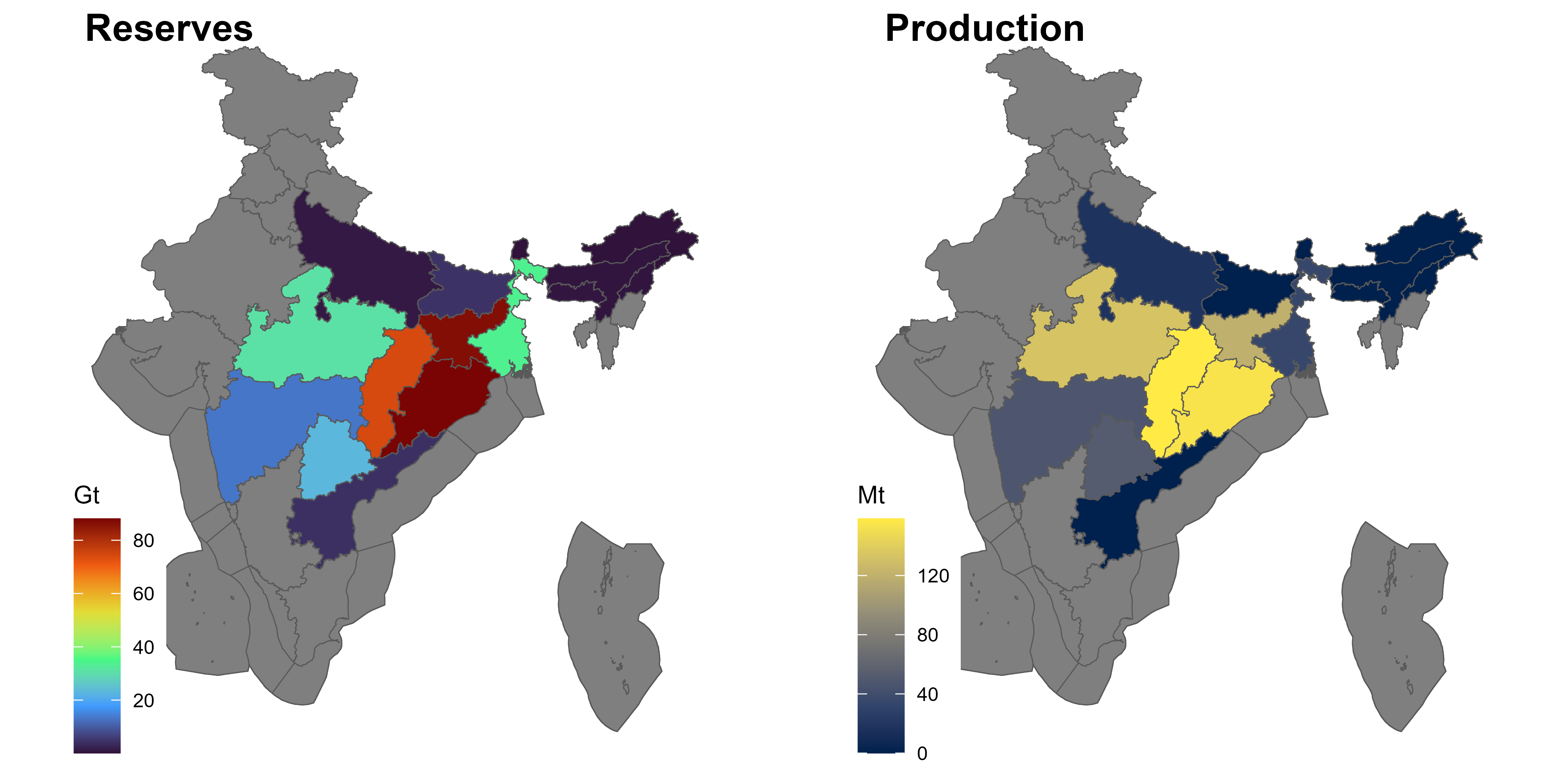

Total coal reserves and production in 2021 by state

Oil

Oil and gas are pivotal within the energy mix, constituting over one-third of the energy requirements due to economic growth and population increase driving up demand annually. In 2020-21, crude oil production stood at 30.49 million metric tons (MMT). India’s imports included 196.46 MMT of crude oil valued at Rs 459,779 crores, 43.25 MMT of petroleum products at Rs 109,430 crores, and 24.8 MMT of liquefied natural gas (LNG) costing Rs 54,850 crores. These imports accounted for 21.4% of the country’s total imports for the year. Conversely, the export of petroleum products reached 56.77 MMT, with a value of Rs 157,168 crores.

code

# loading and processing oil data
# get_ideea_data(name = "oil", raw = T) # check
oil_sup <- 
  get_ideea_data(
    name = "oil", nreg = nreg, variable = "reserve", agg_fun = sum
    ) |>
  full_join(get_ideea_data(
    name = "oil", nreg = nreg, variable = "cost", agg_fun = mean
    ), by = regN) |>
  filter(oil_reserve_GWh_2021 > 0)

# Declaration of commodity
OIL <- newCommodity(
  name = "OIL", 
  desc = "Oil and products",
  unit = "GWh", 
  #slice = "ANNUAL",
  timeframe = "ANNUAL",
  emis = data.frame(
    comm = "CO2",
    unit = "kt/GWh",
    emis = 0.25 # emissions from combustion of 1 unit
  ),
  misc = list(
    emis_source = "https://www.eia.gov/environment/emissions/co2_vol_mass.php",
    emis_conv = 'convert("kg/MMBtu", "kt/GWh", 74)'
  )
)

# Declaration of domestic supply
SUP_OIL <- newSupply(
  name = "SUP_OIL",
  desc = "Domestic oil supply",
  commodity = "OIL",
  unit = "GWh",
  region = unique(oil_sup[[regN]]),
  reserve = data.frame(
    region = oil_sup[[regN]],
    res.up = oil_sup$oil_reserve_GWh_2021
  ),
  availability = data.frame(
    region = oil_sup[[regN]],
    ava.up = oil_sup$oil_reserve_GWh_2021 / 30, # assumption
    cost = convert("USD/kWh", "cr.INR/GWh", oil_sup$oil_cost_USD_kWh)
  )
)

# Declaration of import from other countries, 
# makes supply of oil available in any region
IMP_OIL <- newImport(
  name = "IMP_OIL",
  desc = "Import of oil from abroad",
  commodity = "OIL",
  unit = "GWh",
  imp = data.frame(
    # region = NA, # all regions
    price = 2 * mean(SUP_OIL@availability$cost, na.rm = T) # assuming double costs
  )
)

# saving the model objects in repository
repo_energy <- add(repo_energy, OIL, SUP_OIL, IMP_OIL)
repo_energy |> summary()
#> commodity    import    supply 
#>         2         2         2
repo_energy |> names()
#> [1] "COA"     "SUP_COA" "IMP_COA" "OIL"     "SUP_OIL" "IMP_OIL"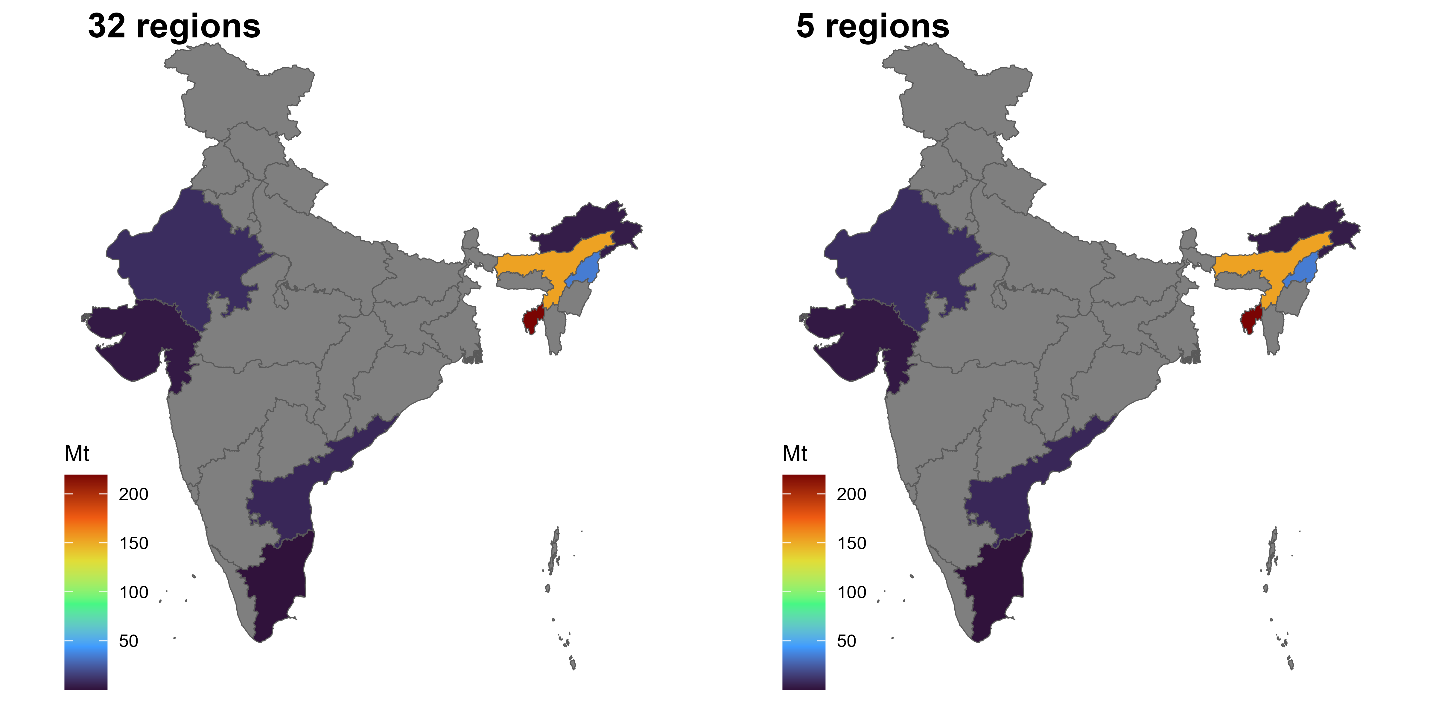

Total oil reserves by region

Gas

Government of India is determined to promote usage of natural gas, as a fuel and feedstock across the country, and to increase its share in primary energy mix from around 6.7% to 15% by 2030 [1]. The estimated CBM resources are of the order of 2600 BCM or 91 Trillion TCF spread over 11 states of the country. Natural Gas Production during 2020-21 stood at 28.67 BCM. Currently, 2575 sq. kms of CBM resources are available in India. Out of 280.357 BCM of CBM, 112.63 BCM of CBM are recoverable reserves [2].

code

# loading and processing oil data
get_ideea_data(name = "gas", raw = T) # check raw data
#>      reg36 reg36_off   reg1 offshore                 name36  name1
#>     <char>    <char> <char>   <lgcl>                 <char> <char>
#>  1:     AP        AP    IND    FALSE         Andhra Pradesh  India
#>  2:     AP    AP_off    IND     TRUE         Andhra Pradesh  India
#>  3:     AR        AR    IND    FALSE      Arunachal Pradesh  India
#>  4:     AS        AS    IND    FALSE                  Assam  India
#>  5:     BR        BR    IND    FALSE                  Bihar  India
#>  6:     CH        CH    IND    FALSE             Chandigarh  India
#>  7:     CT        CT    IND    FALSE           Chhattisgarh  India
#>  8:     DD        DD    IND    FALSE          Daman and Diu  India
#>  9:     DD    DD_off    IND     TRUE          Daman and Diu  India
#> 10:     DL        DL    IND    FALSE                  Delhi  India
#> 11:     DN        DN    IND    FALSE Dadra and Nagar Haveli  India
#> 12:     GA        GA    IND    FALSE                    Goa  India
#> 13:     GA    GA_off    IND     TRUE                    Goa  India
#> 14:     GJ        GJ    IND    FALSE                Gujarat  India
#> 15:     GJ    GJ_off    IND     TRUE                Gujarat  India
#> 16:     HP        HP    IND    FALSE       Himachal Pradesh  India
#> 17:     HR        HR    IND    FALSE                Haryana  India
#> 18:     JH        JH    IND    FALSE              Jharkhand  India
#> 19:     JK        JK    IND    FALSE      Jammu and Kashmir  India
#> 20:     KA        KA    IND    FALSE              Karnataka  India
#> 21:     KA    KA_off    IND     TRUE              Karnataka  India
#> 22:     KL        KL    IND    FALSE                 Kerala  India
#> 23:     KL    KL_off    IND     TRUE                 Kerala  India
#> 24:     MH        MH    IND    FALSE            Maharashtra  India
#> 25:     MH    MH_off    IND     TRUE            Maharashtra  India
#> 26:     ML        ML    IND    FALSE              Meghalaya  India
#> 27:     MN        MN    IND    FALSE                Manipur  India
#> 28:     MP        MP    IND    FALSE         Madhya Pradesh  India
#> 29:     MZ        MZ    IND    FALSE                Mizoram  India
#> 30:     NL        NL    IND    FALSE               Nagaland  India
#> 31:     OR        OR    IND    FALSE                 Odisha  India
#> 32:     OR    OR_off    IND     TRUE                 Odisha  India
#> 33:     PB        PB    IND    FALSE                 Punjab  India
#> 34:     PY        PY    IND    FALSE             Puducherry  India
#> 35:     PY    PY_off    IND     TRUE             Puducherry  India
#> 36:     RJ        RJ    IND    FALSE              Rajasthan  India
#> 37:     SK        SK    IND    FALSE                 Sikkim  India
#> 38:     TG        TG    IND    FALSE              Telangana  India
#> 39:     TN        TN    IND    FALSE             Tamil Nadu  India
#> 40:     TN    TN_off    IND     TRUE             Tamil Nadu  India
#> 41:     TR        TR    IND    FALSE                Tripura  India
#> 42:     UP        UP    IND    FALSE          Uttar Pradesh  India
#> 43:     UT        UT    IND    FALSE            Uttarakhand  India
#> 44:     WB        WB    IND    FALSE            West Bengal  India
#> 45:     WB    WB_off    IND     TRUE            West Bengal  India
#>      reg36 reg36_off   reg1 offshore                 name36  name1
#>     gas_reserve_Bcm_2021 gas_reserve_GWh_2021 gas_cost_USD_kWh
#>                    <num>                <num>            <num>
#>  1:                65.50               695028             0.03
#>  2:                   NA                   NA               NA
#>  3:                 3.14                33319             0.03
#>  4:               166.63              1768129             0.03
#>  5:                   NA                   NA               NA
#>  6:                   NA                   NA               NA
#>  7:                   NA                   NA               NA
#>  8:                   NA                   NA               NA
#>  9:                   NA                   NA               NA
#> 10:                   NA                   NA               NA
#> 11:                   NA                   NA               NA
#> 12:                   NA                   NA               NA
#> 13:                   NA                   NA               NA
#> 14:                56.79               602605             0.03
#> 15:                   NA                   NA               NA
#> 16:                   NA                   NA               NA
#> 17:                   NA                   NA               NA
#> 18:                   NA                   NA               NA
#> 19:                   NA                   NA               NA
#> 20:                   NA                   NA               NA
#> 21:                   NA                   NA               NA
#> 22:                   NA                   NA               NA
#> 23:                   NA                   NA               NA
#> 24:                   NA                   NA               NA
#> 25:                   NA                   NA               NA
#> 26:                   NA                   NA               NA
#> 27:                   NA                   NA               NA
#> 28:                   NA                   NA               NA
#> 29:                   NA                   NA               NA
#> 30:                 0.09                  955             0.03
#> 31:                   NA                   NA               NA
#> 32:                   NA                   NA               NA
#> 33:                   NA                   NA               NA
#> 34:                   NA                   NA               NA
#> 35:                   NA                   NA               NA
#> 36:                59.06               626692             0.03
#> 37:                   NA                   NA               NA
#> 38:                   NA                   NA               NA
#> 39:                37.89               402055             0.03
#> 40:                   NA                   NA               NA
#> 41:                29.18               309632             0.03
#> 42:                   NA                   NA               NA
#> 43:                   NA                   NA               NA
#> 44:                   NA                   NA               NA
#> 45:                   NA                   NA               NA
#>     gas_reserve_Bcm_2021 gas_reserve_GWh_2021 gas_cost_USD_kWh
gas_reserve <- get_ideea_data(name = "gas", nreg = nreg, 
                              variable = "reserve", agg_fun = sum)
gas_ava_assumption <- get_ideea_data(name = "gas_ava_assumption", 
                                     nreg = nreg, 
                                     variable = "ava.up", agg_fun = sum) |>
  left_join(
    get_ideea_data(name = "gas_ava_assumption", 
                   nreg = nreg, 
                   variable = "cost", agg_fun = mean)
  ) 

# Declaration of commodity
GAS <- newCommodity(
  name = "GAS", 
  desc = "Natural gas, all types",
  unit = "GWh", 
  #slice = "ANNUAL", deprecated
  timeframe = "ANNUAL",
  emis = data.frame(
    comm = "CO2",
    unit = "kt/GWh",
    emis = 0.18 # emissions from combustion of 1 unit 
  ),
  misc = list(
    emis_source = "https://www.eia.gov/environment/emissions/co2_vol_mass.php",
    emis_conv = 'convert("kg/MMBtu", "kt/GWh", 53)'
  )
)

# Declaration of domestic supply
SUP_GAS <- newSupply(
  name = "SUP_GAS",
  desc = "Domestic natural supply",
  commodity = "GAS",
  unit = "GWh",
  region = unique(gas_ava_assumption[[regN]]),
  reserve = data.frame(
    region = gas_reserve[[regN]],
    res.up = gas_reserve$gas_reserve_GWh_2021 
  ) |> unique(),
  availability = data.frame(
    region = gas_ava_assumption[[regN]],
    year = gas_ava_assumption$year,
    ava.up = gas_ava_assumption$ava.up,
    cost = gas_ava_assumption$cost
  )
)

# Declaration of import from other countries,
# (makes supply of oil available in any region)
IMP_GAS <- newImport(
  name = "IMP_GAS",
  desc = "Import of natural gas from abroad",
  commodity = "GAS",
  unit = "GWh",
  imp = data.frame(
    # region = NA, # all regions
    #price = 2 * mean(SUP_GAS@availability$cost, na.rm = T) # assuming double costs
    price = 100 * mean(SUP_GAS@availability$cost, na.rm = T) # assuming high costs
  )
)

# saving the model objects in repository
repo_energy <- add(repo_energy, GAS, SUP_GAS, IMP_GAS, overwrite = T)
repo_energy@data |> names()
#> [1] "COA"     "SUP_COA" "IMP_COA" "OIL"     "SUP_OIL" "IMP_OIL" "GAS"    
#> [8] "SUP_GAS" "IMP_GAS"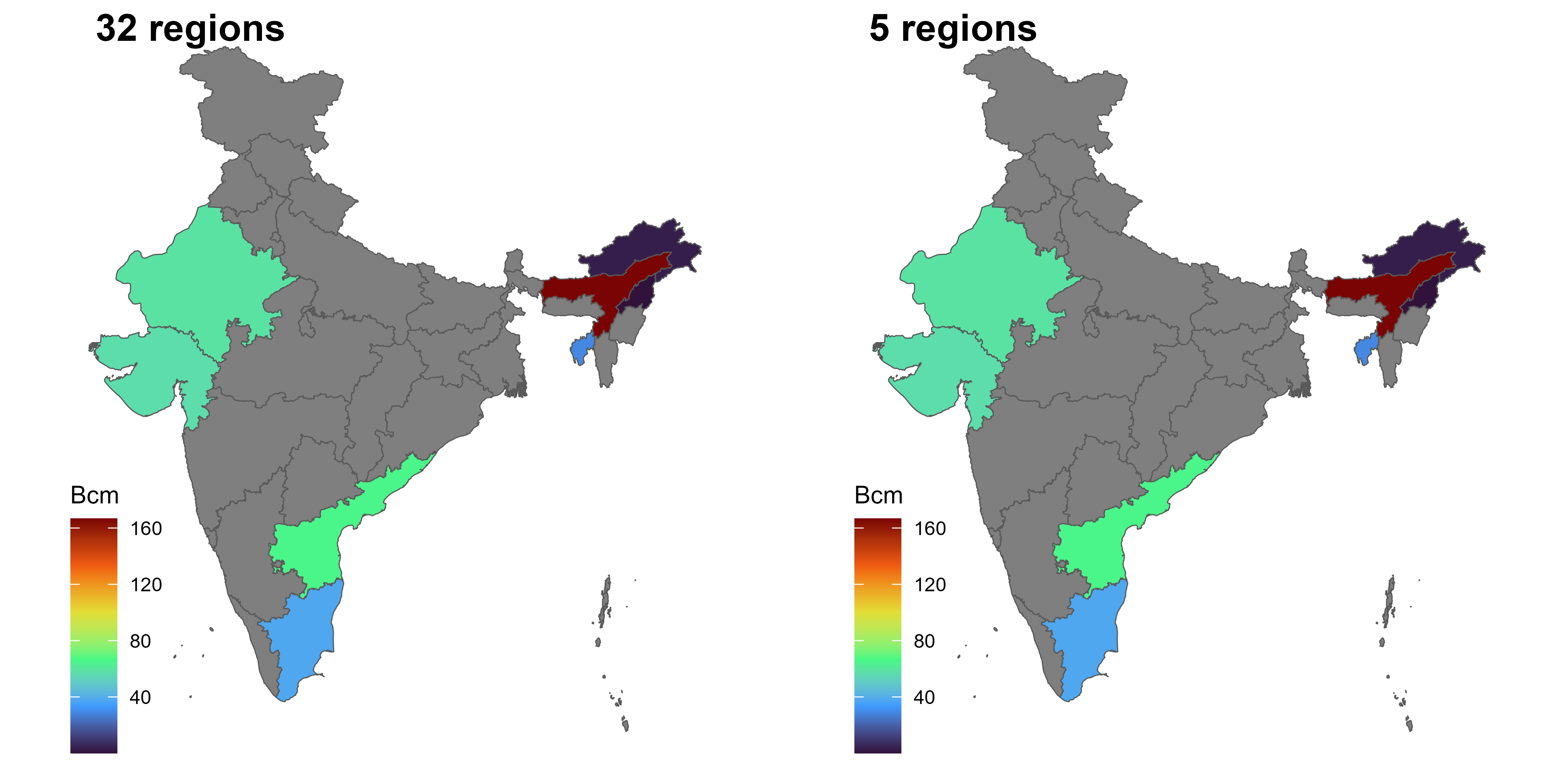

Total gas reserves by region

CCS

Source: Carbon Capture, Utilization and Storage (CCUS) Policy Framework and its Deployment Mechanism in India Utilization and Storage (CCUS)
https://www.niti.gov.in/sites/default/files/2022-11/CCUS-Report.pdf

code

# Data on the potential of CO2 storage in geological formations
# NOTE: the original data is by 5 regions, disaggregation is used for higher nreg
ccs_reserve <- get_ideea_data(name = "ccs_r5", nreg = nreg)

# Declaration of domestic supply
# A commodity to represent the storage of CO2
CO2SINK <- newCommodity(
  name = "CO2SINK", 
  desc = "Stored CO2 in geological formations",
  unit = "kt", 
  timeframe = "ANNUAL"
)

# Declaration of domestic carbon sink resources
RES_CO2SINK <- newSupply(
  name = "RES_CO2SINK",
  desc = "Permanent geological carbon storage (saline aquifers and basalt).",
  commodity = "CO2SINK",
  unit = "kt",
  region = unique(ccs_reserve[[regN]]),
  reserve = data.frame(
    region = ccs_reserve[[regN]],
    res.up = ccs_reserve$CCS_potential_GtCO2 * 1e6
  ) |> unique(),
  availability = list(
    # represent injection costs per unit of stored CO2
    cost = convert(12.1, "USD/t", "cr.₹/kt") # ~0.1 cr.₹/kt, assumption
  )
)

# Saving the model objects in repository
repo_energy <- add(repo_energy, CO2SINK, RES_CO2SINK, overwrite = F)
repo_energy@data |> names()
#>  [1] "COA"         "SUP_COA"     "IMP_COA"     "OIL"         "SUP_OIL"    
#>  [6] "IMP_OIL"     "GAS"         "SUP_GAS"     "IMP_GAS"     "CO2SINK"    
#> [11] "RES_CO2SINK"

Bio

The Centre for Energy Studies Report assesses biomass power and bagasse cogeneration potential in India, covering the gross cropped area from 2015 to 2018, which was about 198.11 million hectares across different seasons. The period saw a production of approximately 774.38 million tonnes from selected crops, leading to an estimated biomass potential of 754.50 million tonnes after applying crop-specific Crop Residue Ratios (CRR). A significant portion (two-thirds, or 525.98 million tonnes) of this biomass is used for domestic purposes, leaving a surplus of 228.52 million tonnes.

This surplus biomass could generate an estimated 28.5 GWe of power, with the major contributions from states like Punjab, Uttar Pradesh, Gujarat, Maharashtra, Madhya Pradesh, and Andhra Pradesh. Future projections for biomass power potential, based on trends from 2015 to 2018, suggest an increase to 30,883.21 MWe by 2020-21, 32,937.83 MWe by 2025-26, and 35,994.52 MWe by 2030-31. This growth in biomass power potential could result from expanded agricultural areas, changes in crop patterns, or improved utilization of residual biomass.

code

# loading and processing data
# get_ideea_data(name = "biomass", raw = T) # check raw data
bio_sup <- get_ideea_data(name = "biomass", 
                          nreg = nreg, 
                          variable = "max_MWe") |>
  filter(max_MWe > 0) |>
  mutate(
    
  )

# bio_ava <- 
#   get_ideea_data("biomass_ava_assumption", nreg = nreg, 
#                  variable = "ava.up", agg_fun = sum) |>
#   full_join(
#     get_ideea_data("biomass_ava_assumption", nreg = nreg, 
#                    variable = "cost", agg_fun = mean)
#     )

# Declaration of commodity
BIO <- newCommodity(
  name = "BIO", 
  desc = "Biomass, all types",
  unit = "GWh", 
  timeframe = "ANNUAL",
  emis = data.frame(
    comm = "PM25",
    unit = "kt/GWh",
    emis = 0.1
  )
)

# Declaration of domestic supply
RES_BIO <- newSupply(
  name = "RES_BIO",
  desc = "Local biomass resource",
  commodity = "BIO",
  unit = "GWh",
  availability = data.frame(
    region = bio_sup[[regN]],
    # year = bio_sup$year,
    ava.up = bio_sup$max_MWe / 1e3 * 8760 * 0.5, # assume 50% CF
    cost = 0.247934 # assumption convert(0.247934, "cr.INR/GWh", "USD/kWh")
  ),
  # availability = data.frame(
  #   region = bio_ava[[regN]],
  #   year = bio_ava$year,
  #   ava.up = bio_ava$ava.up,
  #   cost = bio_ava$cost
  # ),
  region = unique(bio_sup[[regN]])
)

# saving the model objects in repository
repo_energy <- add(repo_energy, BIO, RES_BIO)
repo_energy@data |> names()
#>  [1] "COA"         "SUP_COA"     "IMP_COA"     "OIL"         "SUP_OIL"    
#>  [6] "IMP_OIL"     "GAS"         "SUP_GAS"     "IMP_GAS"     "CO2SINK"    
#> [11] "RES_CO2SINK" "BIO"         "RES_BIO"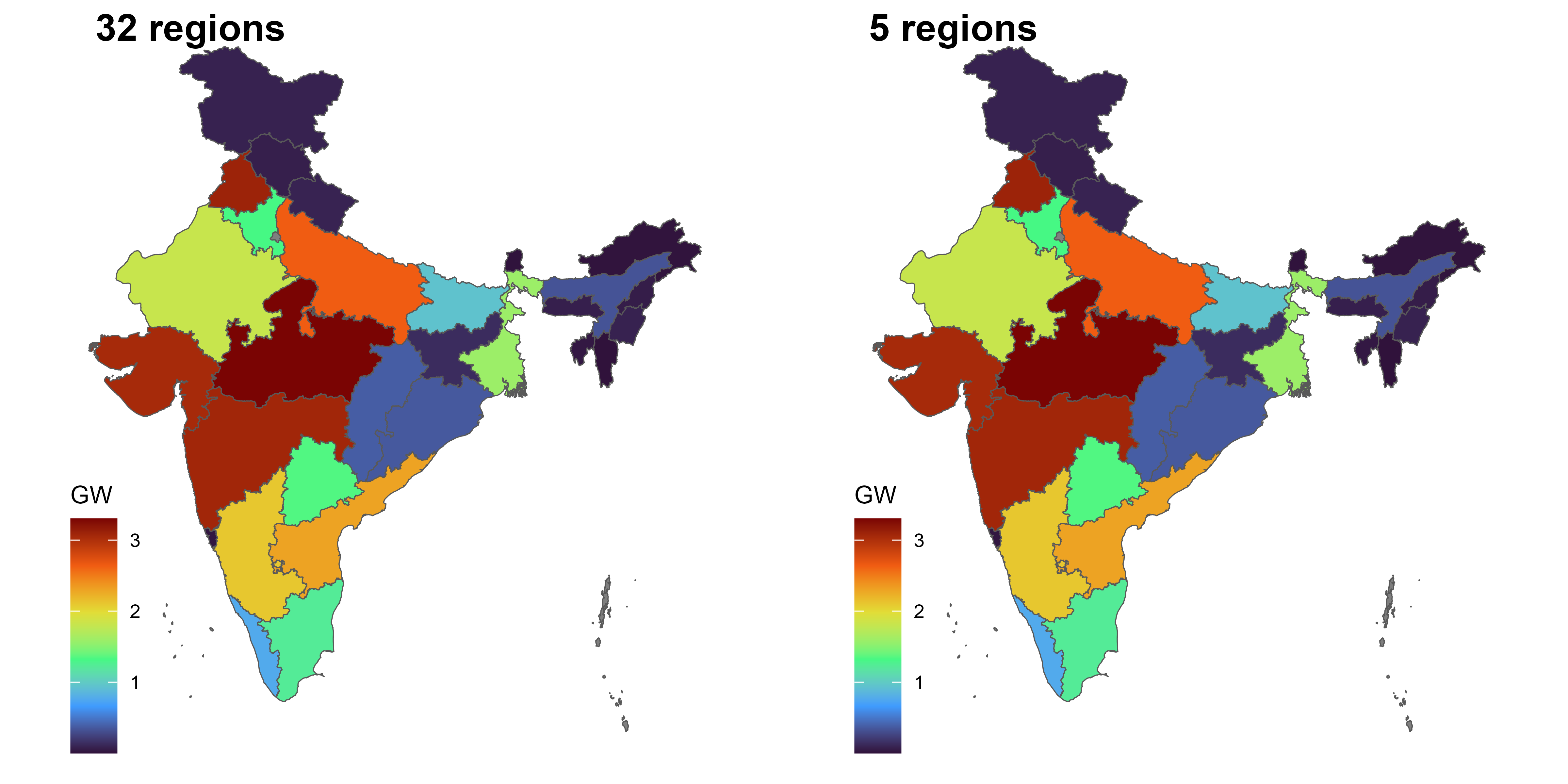

Total bio reserves by region

Wind

As per National Institute of Wind Energy (NIWE), installable wind potential in India at 50 m, 80m, 100 m and 120m above the ground level are 49 GW, 103 GW and 302 GW respectively [2, 3]. The commercially exploitable wind potential is more than 200 GW. Currently, total installed capacity of wind in India is around 41 GW i.e., 20% of the total commercially exploitable potential [4]. Tamil Nādu, Gujarat, Karnataka, Rajasthan & Maharashtra are the top 5 wind energy potential states [5]. India is also blessed with 7600 km of coast line and estimated off-shore wind potential is around 194 GW. Coastal area of Gujarat and coastline of Rameshwaram and Kanyakumari offer offshore wind potential which is almost around 71GW [6, 7]. The wind speed is available at the above-mentioned coastal areas is around 7 m/s – 9m/s [8]. The capital cost of investment required for 1 MW of wind power plant installation is around 5 – 5.5 Crores and the levelized cost of generation is around INR 2-3. [9].

ideea_cl_sf <- get_ideea_cl_sf(resource = "win", tol = 0.05) |>
# plot(ideea_cl_sf["MW_max"])
# ideea_cl_sf |> 
  group_by(across(any_of(
    c(regN, regN_off, "mainland", "offshore", "cluster"))
    )) |>
  summarise(
    MW_max = sum(MW_max),
    geometry = sf::st_union(geometry)
  )

ggplot() +
  geom_sf(data = ideea_sf) +
  geom_sf(aes(fill = MW_max/1e3), data = ideea_cl_sf) +
  scale_fill_viridis_c(option = "H", name = "GW") +
  theme_map()

Solar

Solar power Generation in India is 67 GW[6] which accounts for 16% of the total power generation in India. In the Financial Year of 2022-23, a total of 102 Billion Units[7] of Solar power was generated. The total potential for solar power in India is estimated to be 748GW. However any estimates of solar power are based on used land assumptions and the current state of the technology. With

The National Solar Mission was launched in 2010 to promote ecological sustainable growth while addressing India’s energy security challenges. It will also constitute a major contribution by India to the global effort to meet the challenges of climate change. The Mission’s objective is to establish India as a global leader in solar energy by creating the policy conditions for solar technology diffusion across the country as quickly as possible.[11] The policy had a target of 100 GW installed capacity of Solar power in India by 2022, but has achieved installed capacity of 62GW in 2022. It is estimated that by 2026, 100 GW of solar power will be installed and India can become a net exporter of Solar power[12].

Hydro

In India, hydroelectric plants are categorised as large hydro (>25MW) and small hydro (≤25MW). Government authorities conduct periodic studies on estimating the potential of large hydro plants. Data on large hydro potential, capacity in operation and capacity under construction till March 2023 have been collated from [https://pib.gov.in/PressReleasePage.aspx?PRID=1909276] and installed capacity of small hydro plants till June 2023 have been obtained from [https://mnre.gov.in/img/documents/uploads/file_s-1689077131891.pdf]. Construction of hydro projects typically involve long construction periods due to sites being prone to geological surprises. This makes it difficult to determine a unified levelized price and it varies from project to project. However, for the large hydro projects installed in the last few years, the average price has been observed to work out as INR 5.42 per kWh [https://energy.economictimes.indiatimes.com/news/power/reviving-indias-sleeping-energy-giant-hydro-pumped-hydro-power/97294420]

Nuclear

summarize existing and planned projects
normally not included to optimization
https://www.world-nuclear.org/information-library/country-profiles/countries-g-n/india.aspx

code

# Declaration of commodity
NUC <- newCommodity(
  name = "NUC", 
  desc = "Nuclear fuel",
  unit = "GWh", 
  #slice = "ANNUAL" deprecated
  timeframe = "ANNUAL"
)

IMP_NUC <- newImport(
  name = "IMP_NUC",
  desc = "Import of nuclear fuel",
  commodity = "NUC",
  unit = "GWh",
  imp = data.frame(
    # region = NA, # all regions
    price = convert("cents/kWh", "cr.INR/GWh", 0.46 * .35) 
    # price adjusted for 35% efficiency
  ),
  misc = list(
    source = "https://world-nuclear.org/information-library/economic-aspects/economics-of-nuclear-power.aspx",
    cost = "fuel cost = 0.46 ¢/kWh"
  )
)

# saving the model objects in repository
repo_energy <- add(repo_energy, NUC, IMP_NUC, overwrite = F)
repo_energy@data |> names()
#>  [1] "COA"         "SUP_COA"     "IMP_COA"     "OIL"         "SUP_OIL"    
#>  [6] "IMP_OIL"     "GAS"         "SUP_GAS"     "IMP_GAS"     "CO2SINK"    
#> [11] "RES_CO2SINK" "BIO"         "RES_BIO"     "NUC"         "IMP_NUC"

Settings

Coal and Lignite

Definition of commodity and supply

Oil

Gas

CCS

Bio

Wind

Solar

Hydro

Nuclear

References