Karnataka electric power sector capacity expansion model

library(IDEEA)
library(data.table)
library(tidyverse)
library(ggrepel)
library(fst)

Configuration

tmz <- "Asia/Kolkata" # model timezone
baseYear <- 2019 # model base year
# modYears <- c(baseYear + c(0, 2), seq(2025, 2060, by = 5)) # model years
# weaYears <- 2019 # weather years (from MERRA-2)

# Currency conversion
INR_Crore_2_USD <- 136825.20 # Google converter, Jan 13, 2021
INR_2_USD <- INR_Crore_2_USD / 1e7
INR_Crore_2_MUSD <- INR_Crore_2_USD/1e6 
INR_Lakh_2_MUSD <- INR_Crore_2_MUSD/100

ideea_sf <- get_ideea_map(nreg = 32, offshore = FALSE, ROW = FALSE, rename = TRUE)
karnataka_sf <- ideea_sf[ideea_sf$region == "KA", ]

plot(ideea_sf["region"], col = NA, reset = F, main = "Karnataka")
plot(karnataka_sf["region"], col = "red", add = T)

Weather classes

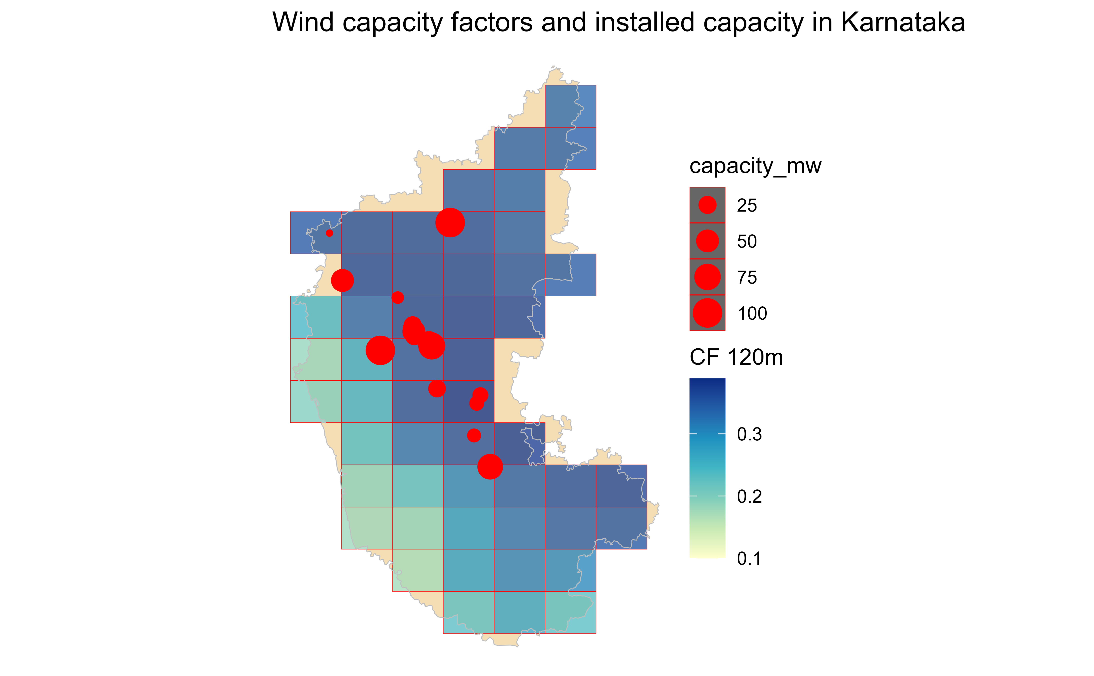
Wind (by resource class)

# generating capacity
gen_cap <- ideea_data$karnataka$capacity_MW
# wind capacity factors
wind_cf <- ideea_data$karnataka$wind_cf
# wind and solar average potential estimates
merra_CF_mean <- ideea_data$karnataka$merra_CF_mean
# wind_loc_sf <- ideea_data$karnataka$wind_loc_sf

(wind_120m <- unique(merra_CF_mean$af120m_class))
#> [1] "AF20" "AF25" "AF15" "AF30" "AF35"
ww <- merra_CF_mean$af120m_class %in% wind_120m
ggplot(karnataka_sf) +
  geom_sf(aes(),
    fill = "wheat",
    colour = "white", alpha = 1, size = .5, show.legend = F
  ) + 
  theme_void() +
  # ggplot(merra_CF_mean[ww,]) +
  geom_tile(aes(lon, lat, fill = af120m),
    data = merra_CF_mean,
    inherit.aes = F, alpha = .75, show.legend = T
  ) +
  scale_fill_distiller(
    palette = "YlGnBu", name = "CF 120m", direction = 1,
    limits = c(0.1, NA), na.value = "grey70"
  ) +
  geom_tile(aes(lon, lat),
    data = merra_CF_mean[ww, ], 
    colour = "red", fill = NA,
    inherit.aes = F, show.legend = T
  ) +
  geom_sf(fill = NA, colour = "grey", alpha = 1, size = .5, 
          data = karnataka_sf) + 
  geom_point(aes(lon, lat, size = capacity_mw),
             colour = "red",
             data = ideea_data$karnataka$wind_loc_sf, 
             inherit.aes = FALSE) +
  labs(
    title = "Wind capacity factors and installed capacity in Karnataka"
    # subtitle = "Wind resource classes and potential locations",
    # caption = "Source: MERRA-2, WRI, IDEEA"
  )

  # theme_ideea_map()
  

# Create weather-class for every AF-type of the resource
summary(wind_cf$wcf_120m)
#>    Min. 1st Qu.  Median    Mean 3rd Qu.    Max. 
#> 0.01405 0.21568 0.36705 0.35481 0.47791 0.75000
WWIN_120m <- newRepository("WWIN_120m")
for (i in wind_120m) {
  ii <- wind_cf$af120m_class == i
  WWIN_i <- newWeather(
    name = paste0("WWIN_", i),
    # desc = "",
    # unit = "kWh/kWh_max",
    timeframe = "HOUR",
    weather = data.frame(
      # region = as.character(),
      # year = merra_CF_mean$mYear[ii],
      slice = wind_cf$slice[ii],
      wval = wind_cf$wcf_120m[ii] 
    )
  )
  WWIN_120m <- add(WWIN_120m, WWIN_i)
}
names(WWIN_120m@data)
#> [1] "WWIN_AF20" "WWIN_AF25" "WWIN_AF15" "WWIN_AF30" "WWIN_AF35"

Solar (regional average)

# solar average capacity factors
solar_cf <- ideea_data$karnataka$solar_cf

# Create weather-class for solar resource (average)
summary(solar_cf$scf)
#>    Min. 1st Qu.  Median    Mean 3rd Qu.    Max. 
#> 0.00000 0.00000 0.01139 0.24138 0.48715 1.00000
WSOL_mean <- newWeather(
  name = "WSOL",
  # desc = "",
  # unit = "kWh/kWh_max",
  timeframe = "HOUR",
  weather = data.frame(
    slice = solar_cf$slice,
    wval = solar_cf$scf 
  )
)

# gen_cap$cap_MW[grepl("Solar", gen_cap$enSource)] / 1e3 *
#   sum(merra_sol_mean$afsol)

Hydro (reservoirs inflows)

# Inflow and discharge data of reservoirs
w_hyd <- ideea_data$karnataka$reservoir |>
  filter(year(datetime) %in% baseYear) %>%
  mutate(date = as_date(datetime)) %>%
  ungroup() %>%
  dplyr::select(-datetime) %>%
  mutate(slice = dtm2tsl(date, format = "d365"))
w_hyd[c(1, nrow(w_hyd)),] # accumulated energy -first and last days of the year
#>    DISCHARGE_MU EQENERGY_MU INFLOW_MU       date  slice
#>           <num>       <num>     <num>     <Date> <char>
#> 1:    -28.19596    6133.078  2.625201 2019-01-01   d001
#> 2:    -33.75062    7136.870  8.159480 2019-12-31   d365
sum(w_hyd$INFLOW_MU) # total inflow
#> [1] 9773.639
sum(w_hyd$DISCHARGE_MU) # total discharge (!some days are missing in the data-Adjusting Coefficient)
#> [1] -8006.358

# Adjust the 3-dams data, adding reservoirs with missing info
gen_cap
#> # A tibble: 6 × 6
#>    year enSource   cap_MW  gen_MU     af type      
#>   <dbl> <chr>       <dbl>   <dbl>  <dbl> <chr>     
#> 1  2019 Biomass      134.    86.5 0.0736 biomass   
#> 2  2019 Hydro       4665. 14327.  0.351  hydro     
#> 3  2019 Net_Import  4133. 20562.  0.568  net_import
#> 4  2019 Solar       7038  11524.  0.216  solar     
#> 5  2019 Thermal    10379. 16578.  0.182  thermal   
#> 6  2019 Wind        4778.  8528.  0.204  wind
ii <- grepl("Hydro", gen_cap$enSource)
summary(ii)
#>    Mode   FALSE    TRUE 
#> logical       5       1
gen_cap$gen_MU[ii]
#> [1] 14327.19
sum(w_hyd$INFLOW_MU)
#> [1] 9773.639
(hyd_adj <- gen_cap$gen_MU[ii] / sum(w_hyd$INFLOW_MU)) # Adjusting Coefficient
#> [1] 1.465901

# Hydro   weather class repository 
WHYD_AF <- newWeather("WHYD_AF",
  desc = "Exogenous hydro energy inflow",
  region = "KA",
  timeframe = "YDAY",
  weather = data.frame(
    region = "KA",
    # year = 2010,
    slice = w_hyd$slice,
    wval = w_hyd$INFLOW_MU * hyd_adj # assumption
  )
)

Generating technologies

Thermal

gen_cap
#> # A tibble: 6 × 6
#>    year enSource   cap_MW  gen_MU     af type      
#>   <dbl> <chr>       <dbl>   <dbl>  <dbl> <chr>     
#> 1  2019 Biomass      134.    86.5 0.0736 biomass   
#> 2  2019 Hydro       4665. 14327.  0.351  hydro     
#> 3  2019 Net_Import  4133. 20562.  0.568  net_import
#> 4  2019 Solar       7038  11524.  0.216  solar     
#> 5  2019 Thermal    10379. 16578.  0.182  thermal   
#> 6  2019 Wind        4778.  8528.  0.204  wind
ii <- grepl("Thermal", gen_cap$enSource)
summary(ii)
#>    Mode   FALSE    TRUE 
#> logical       5       1
ECOA <- newTechnology(
  name = "ECOA",
  desc = "Generic Coal-fired power plant, base year",
  # region = ppb$region[ii],
  input = list(
    comm = "COA",
    unit = "GWh",
    combustion = 1
  ),
  output = list(
    comm = "ELC",
    unit = "GWh"
  ),
  cap2act = 24 * 365,
  ceff = list(
    comm = c("COA"),
    cinp2use = c(.35)
  ),
  af = list(
    af.lo = .2, # aggregated lower bound
    rampup = 48, # hours, cold start from 0 to 100, assumption
    rampdown = 48 # assumption
  ),
  afs = list(
    slice = "ANNUAL",
    afs.up = .6, # assumption
    afs.lo = .2 # assumption
  ),
  fixom = list(
    # fixom = .05 * 800 # 5% a year of invcost (800 USD/kW)
    fixom = convert("MUSD/MW", "MUSD/GW", 11.7 * INR_Lakh_2_MUSD)
  ),
  varom = list(
    # varom = 0.01 # USD/kWh - assumption
    # convert("USD/kWh", "MUSD/GWh", 1)
    varom = convert("USD/kWh", "MUSD/GWh", 0.6 * INR_2_USD) 
  ),
  invcost = list(
    invcost = convert("MUSD/MW", "MUSD/GW", 8.02 * INR_Crore_2_MUSD)
  ),
  capacity = data.frame(
    region = "KA",
    year = c(rep(baseYear, sum(ii)), rep(2040, sum(ii))),
    stock = c(gen_cap$cap_MW[ii] / 1e3, 0.7 * gen_cap$cap_MW[ii] / 1e3) # assumption
  ),
  end = list(
    end = 2010
  ),
  olife = list(
    olife = 25
  ),
  timeframe = "HOUR"
)
draw(ECOA)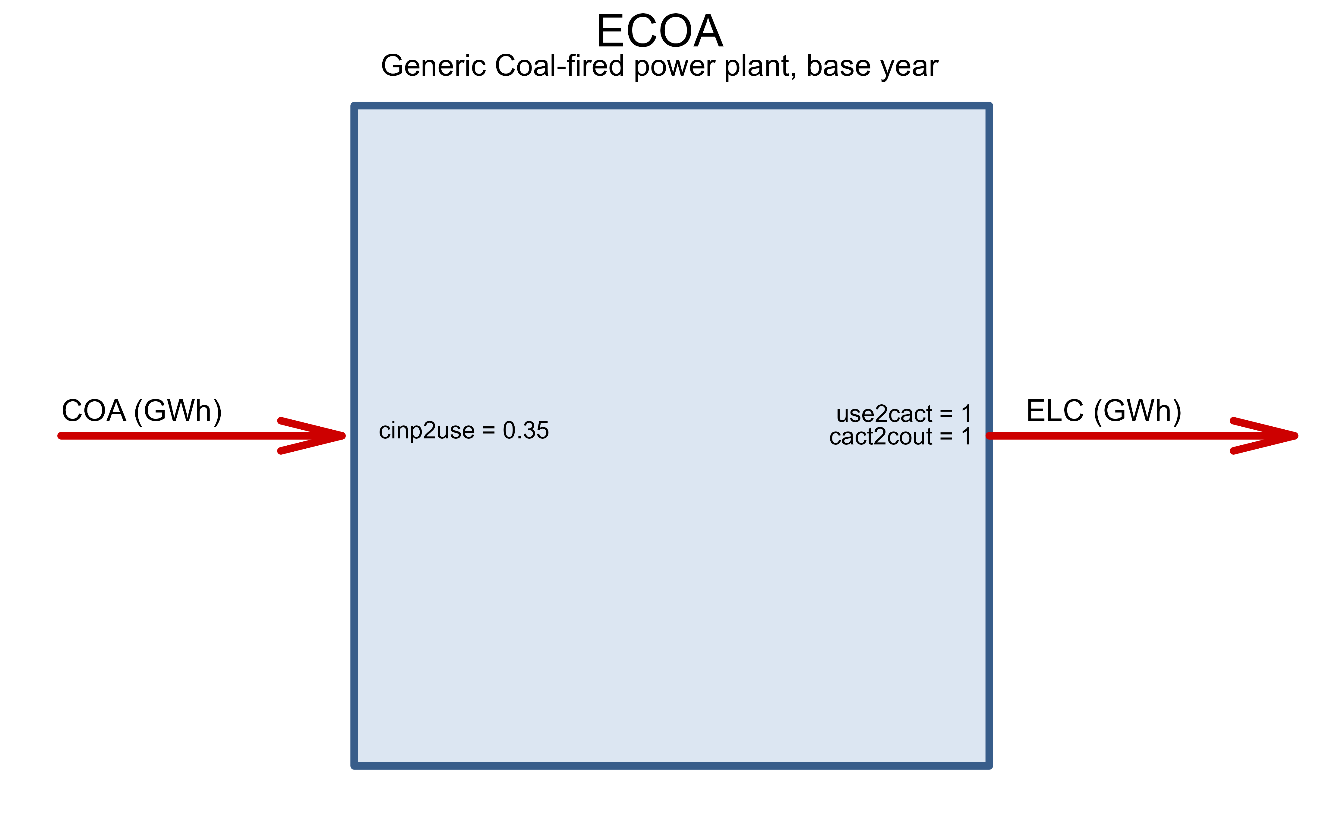

Hydro

ii <- grepl("Hydro", gen_cap$enSource)
stopifnot(sum(ii) == 1) # check
EHYD <- newTechnology(
  name = "EHYD",
  desc = "Hydro power plants",
  # region = ppb$region[ii],
  region = "KA",
  input = list(
    comm = "HYD",
    unit = "GWh",
    combustion = 0
  ),
  output = list(
    comm = "ELC",
    unit = "GWh"
  ),
  # aux = list(acomm = "DAM"),
  cap2act = 24 * 365,
  # ceff = list(
  #   comm = c("HYD"),
  #   cinp2use = c(1)
  # ),
  # aeff = data.frame(
  #   acomm = "DAM",
  #   comm = "HYD",
  #   cinp2ainp  = 1
  # ),
  af = list(
    af.lo = .1, # aggregated lower bound
    # rampup = 4, # hours, cold start from 0 to 100, assumption
    rampdown = 8 # assumption
  ),
  # af = list(
  #   # region = ppb$region[ii],
  #   # slice = ,
  #   af.fx = ppb$af[ii]
  # ),
  fixom = list(
    fixom = convert("MUSD/MW", "MUSD/GW", 20 * INR_Lakh_2_MUSD)
  ),
  # varom = list(
  #   varom =
  # ),
  invcost = list(
    # year = 2010,
    invcost = convert("MUSD/MW", "MUSD/GW", 8.02 * INR_Crore_2_MUSD)
  ),
  capacity = data.frame(
    region = "KA",
    year = c(rep(baseYear, sum(ii)), rep(2060, sum(ii))),
    stock = c(gen_cap$cap_MW[ii] / 1e3, gen_cap$cap_MW[ii] / 1e3)
  ),
  # start = list(
  #   start = 2060
  # ),
  end = list(
    end = 2010
  ),
  olife = list(
    olife = 40
  ),
  timeframe = "HOUR"
)
draw(EHYD)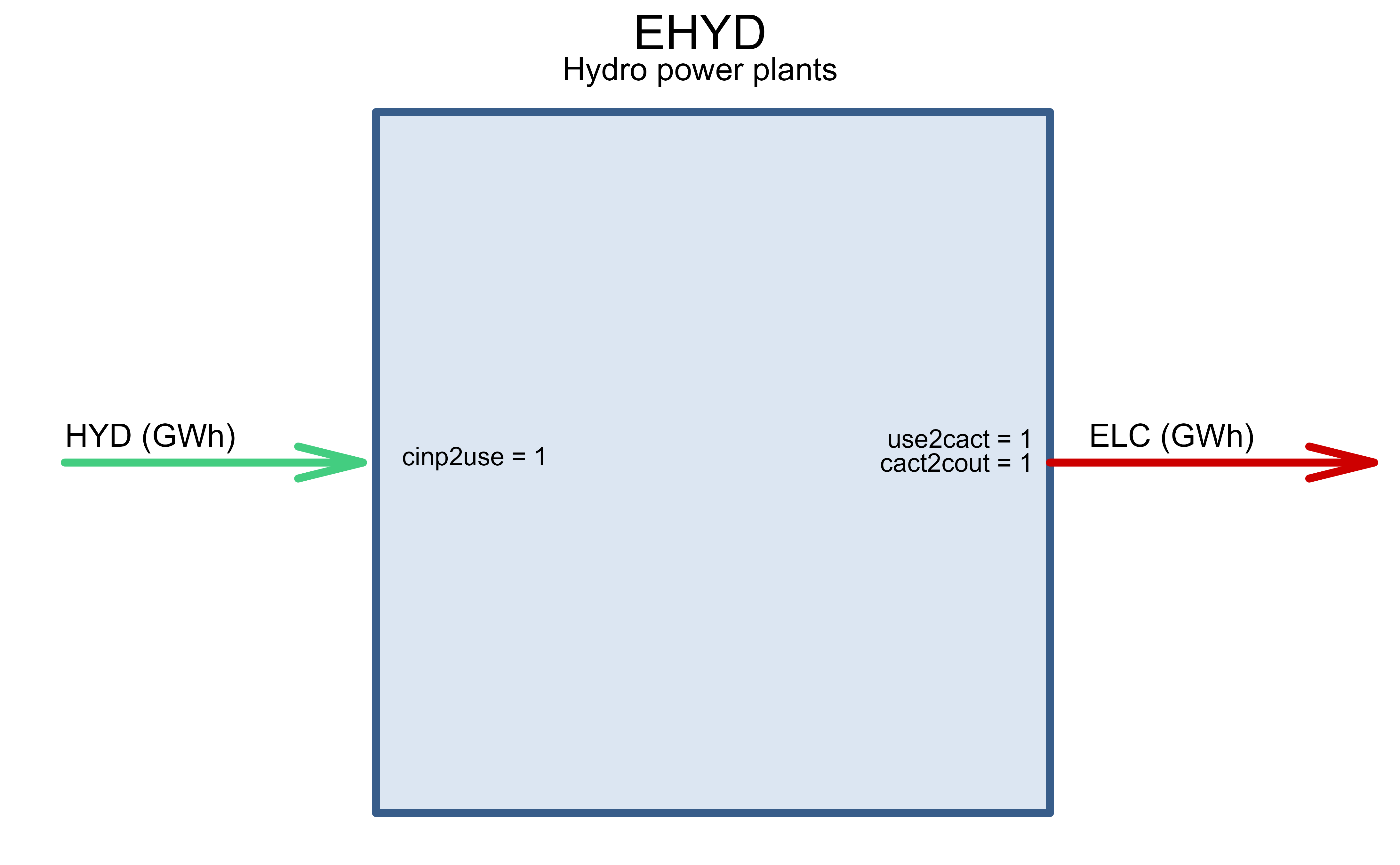

Solar

ii <- grepl("Solar", gen_cap$enSource)
stopifnot(sum(ii) == 1) # check
ESOL <- newTechnology(
  name = "ESOL",
  desc = "Utility Scale Solar PV",
  # region = "AZ",
  input = list(
    comm = "SOL",
    unit = "GWh"
  ),
  output = list(
    comm = "ELC",
    unit = "GWh"
  ),
  cap2act = 365 * 24,
  af = list(
    af.fx = 1 # forcing output when resource is available
  ),
  weather = list(
    weather = "WSOL",
    waf.fx = 1 # weather factor (multiplier) will be applied to af.fx
  ),
  fixom = list(
    # fixom = 10 # assumed, 1% of investment costs a year
    fixom = convert("MUSD/MW", "MUSD/GW", 4.5 * INR_Lakh_2_MUSD)
  ),
  invcost = list(
    # Assuming 1$/Watt
    # https://www.nrel.gov/news/press/2017/nrel-report-utility-scale-solar-pv-system-cost-fell-last-year.html
    # invcost = 1000 # convert("USD/W", "MUSD/GW", 1)
     invcost = convert("MUSD/MW", "MUSD/GW", 3.4 * INR_Crore_2_MUSD)
  ),
  
capacity = data.frame(
    region = "KA",
    year = c(rep(baseYear, sum(ii)), 
             rep(2040, sum(ii)),
             rep(2050, sum(ii))),
    stock = c(gen_cap$cap_MW[ii] / 1e3, 
              0.8 * gen_cap$cap_MW[ii] / 1e3,
              0 * gen_cap$cap_MW[ii])
  ),
  # start = list(
  #   start = 2017
  # ),
  # end = list(end = 2000),
  olife = list(
    olife = 25
  )
)
draw(ESOL)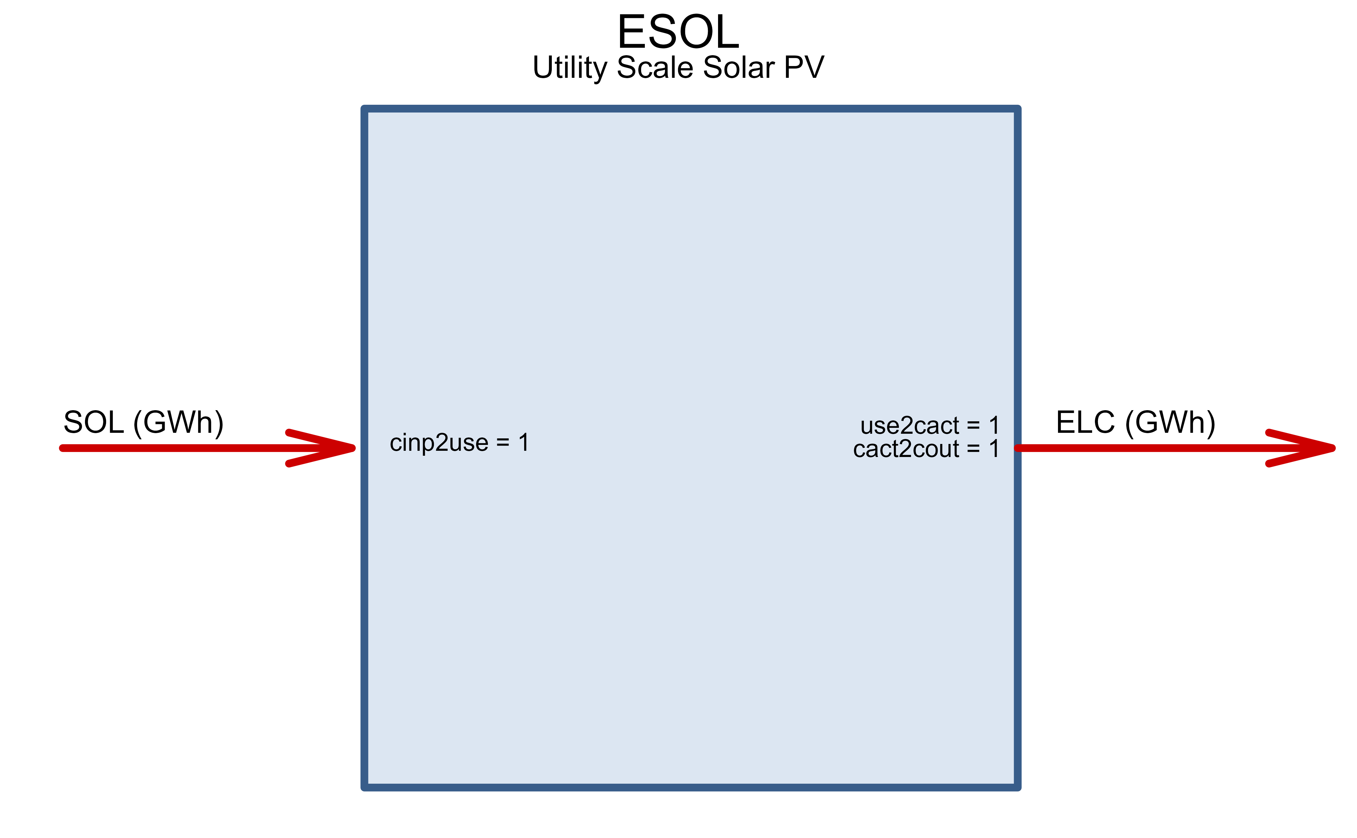


# bulk solar resource
sol_max_GW <- ideea_data$karnataka$solar_max_GW
# Limits on solar total capacity
CSOL_UP <- newConstraintS(
  name = "CSOL_UP",
  eq = "<=",
  type = "capacity",
  for.each = data.frame(
    year = NA,
    tech = "ESOL",
    region = "KA"
    # region = reg_area$region
  ),
  rhs = data.frame(
    # year = modYears,
    tech = "ESOL",
    region = sol_max_GW$region,
    # up to 2% of territory per region
    rhs = 0.02 * round(sol_max_GW$max_GW, 1e-20) 
  ),
  defVal = 1e-20 # to avoid dropping zeros in some solvers
)

Wind

ii <- grepl("Wind", gen_cap$enSource)
summary(ii)
#>    Mode   FALSE    TRUE 
#> logical       5       1
EWIN <- newTechnology(
  name = "EWIN",
  desc = "Onshore wind farm",
  # WIN10_AF@region, # Limiting to regions with available resource
  input = list(
    comm = "WIN",
    unit = "GWh",
    combustion = 0
  ),
  output = list(
    comm = "ELC",
    unit = "GWh"
  ),
  cap2act = 365 * 24,
  af = list(
    af.fx = 1 # forcing output when resource is available
  ),
  weather = list(
    weather = "WWIN", # assumption
    waf.fx = c(1)
    # waf.up = c(1) #
  ),
  fixom = list(
    # fixom = 15 # Assumed, 1% a year
    fixom = convert("MUSD/MW", "MUSD/GW", 8 * INR_Lakh_2_MUSD)
  ),
  invcost = list(
    # Assuming 1.5$/Watt
    # https://www.irena.org/-/media/Files/IRENA/Agency/Publication/2018/Jan/IRENA_2017_Power_Costs_2018.pdf
    # invcost = 1500 #
    invcost = convert("MUSD/MW", "MUSD/GW", 6 * INR_Crore_2_MUSD)
    
  ),
  capacity = data.frame(
    region = "KA",
    year = c(rep(baseYear, sum(ii)), 
             rep(2040, sum(ii)),
             rep(2050, sum(ii))),
    stock = c(gen_cap$cap_MW[ii] / 1e3, 
              0.8 * gen_cap$cap_MW[ii] / 1e3,
              0 * gen_cap$cap_MW[ii])
  ),
  # start = list(
  #   start = 2017
  # ),
  end = list(end = 2000),
  olife = list(
    olife = 25
  )
)
draw(EWIN)


EWIN_120m <- newRepository("EWIN_120m")
for (i in 1:length(WWIN_120m@data)) {
  wName <- WWIN_120m@data[[i]]@name
  tName <- gsub("WWIN_", "EWIN_", wName)
  EWIN_i <- newTechnology(
    name = tName,
    desc = "Utility Scale Solar PV",
    # region = "AZ",
    input = list(
      comm = "SOL",
      unit = "GWh"
    ),
    output = list(
      comm = "ELC",
      unit = "GWh"
    ),
    cap2act = 365 * 24,
    af = list(
      af.fx = 1 # forcing output when resource is available
    ),
    weather = list(
      weather = wName,
      waf.fx = 1 # weather factor (multiplier) will be applied to af.fx
    ),
    # fixom = list(
    #   fixom = 10 # assumed, 1% of investment costs a year
    # ),
    invcost = list(
      # Assuming 1$/Watt
      # https://www.nrel.gov/news/press/2017/nrel-report-utility-scale-solar-pv-system-cost-fell-last-year.html
      invcost = 1000 # convert("USD/W", "MUSD/GW", 1)
    ),
    # start = list(
    #   start = 2017
    # ),
    # end = list(end = 2030),
    olife = list(
      olife = 25
    )
  )
  EWIN_120m <- add(EWIN_120m, EWIN_i)
  # draw(EWIN)
}

# estimated bulk wind resource
win_max_GW <- ideea_data$karnataka$wind_max_GW
# Limits on wind total capacity
CWIN_UP <- newConstraintS(
  name = "CWIN_UP",
  eq = "<=",
  type = "capacity",
  for.each = data.frame(
    year = NA,
    tech = paste0("EWIN_", win_max_GW$af120m_class),
    region = win_max_GW$region
  ),
  rhs = data.frame(
    year = NA,
    tech = paste0("EWIN_", win_max_GW$af120m_class),
    region = win_max_GW$region,
    rhs = 0.1 * round(win_max_GW$max_GW, 1e-20) # up to 10% of territory per region
  ),
  defVal = 1e-20 # to avoid dropping zeros in some solvers
)

Commodities

ELC <- newCommodity("ELC", timeframe = "HOUR")
CO2 <- newCommodity("CO2", timeframe = "ANNUAL")
SOL <- newCommodity("SOL", timeframe = "ANNUAL")
WIN <- newCommodity("WIN", timeframe = "ANNUAL")
WIF <- newCommodity("WIF", timeframe = "ANNUAL")

UHV <- newCommodity(
  name = "UHV",
  desc = "Ultra High Voltage electricity",
  timeframe = "HOUR"
)

COA <- newCommodity(
  name = "COA",
  desc = "All coals",
  # emis = list( #
  #   comm = "CO2", #
  #   unit = "kt/GWh", #
  #   mean = convert("kt/PJ", "kt/GWh", 100) #
  # ),
  timeframe = "ANNUAL"
)

GAS <- newCommodity(
  name = "GAS",
  desc = "Natural gas",
  timeframe = "ANNUAL"
)

BIO <- newCommodity(
  name = "BIO",
  desc = "Biomass",
  timeframe = "ANNUAL"
)

HYD <- newCommodity(
  name = "HYD",
  desc = "Hydro energy",
  timeframe = "YDAY"
)

# DAM <- newCommodity(
#   name = 'DAM',
#   desc = "Hydro energy from Dam", # Auxiliary/artificial
#   timeframe = "YDAY")


NUC <- newCommodity(
  name = "NUC",
  desc = "Nuclear energy",
  timeframe = "ANNUAL"
)

Demand

dem_baseYear <- ideea_data$karnataka$load_curve |>
  filter(year == baseYear)

# projected demand growth
dem_last_year <- dem_baseYear %>%
  mutate(
    year = 2070, 
    MWh = 5 * MWh) # assume 5X growth from 2019 to 2070
dem_modYear <- bind_rows(dem_baseYear, dem_last_year)

#Demand class repository 
DEM_ELC_DH <- newDemand(
  name = "DEM_ELC_DH",
  desc = "Demand by hours and year-days, full year",
  commodity = "ELC",
  unit = "GWh",
  dem = data.frame(
    year = dem_modYear$year,
    region = "KA",
    slice = dem_modYear$slice,
    dem = round(dem_modYear$MWh / 1e3, 3)
  )
)

# Check
dim(DEM_ELC_DH@dem)
#> [1] 17472     4
dim(DEM_ELC_DH@dem)[1] / 365 / 24
#> [1] 1.994521

# DEM_ELC_DH@dem[is.na(DEM_ELC_DH@dem$dem), ] # check for missing values

Supply


RES_SOL <- newSupply(
  name = "RES_SOL",
  desc = "Terrestrial solar radiation",
  commodity = "SOL",
  unit = "GWh"
  # slice = "ANNUAL"
)

RES_WIN <- newSupply(
  name = "RES_WIN",
  desc = "Onshore wind",
  commodity = "WIN",
  # region = unique(wnd_af10$region),
  unit = "GWh"
  # slice = "ANNUAL"
)

# RES_WFF <- newSupply(
#   name = "RES_WFF",
#   desc = "Offshore wind - maximum potential",
#   commodity = "WFF",
#   region = unique(wndf_af10$region),
#   unit = "GWh",
#   slice = "ANNUAL"
# )

RES_HYD <- newSupply(
  name = "RES_HYD",
  desc = "Hydro-resource",
  commodity = "HYD",
  # slice = "YDAY",
  weather = data.frame(
    weather = "WHYD_AF",
    wava.fx = 1
  ),
  availability = list(ava.fx = 1)
)

SUPNUC <- newSupply(
  name = "SUPNUC",
  commodity = "NUC",
  unit = "GWh",
  availability = list(
    # ava.up = convert("GWh", "PJ", 20*24*365),
    # http://www.world-nuclear.org/information-library/economic-aspects/economics-of-nuclear-power.aspx
    cost = convert("USD/kWh", "MUSD/GWh", .39 / 100)
  )
  # slice = "ANNUAL"
)

SUPCOA <- newSupply(
  name = "SUPCOA",
  commodity = "COA",
  desc = "Simplified coal supply",
  availability = list(
    # cost = convert("USD/tce", "MUSD/GWh", 70 / .7)
    cost = convert("USD/tce", "MUSD/GWh", 6000 * INR_2_USD / 0.7) # 0.7 tone -> tce
  )
  # slice = "ANNUAL"
)

# 1,000 Cubic Feet Of Natural Gas to Therms (u.s.) = 10.0024
# 4 USD/cu.ft ~= 0.4 USD/therm
SUPGAS <- newSupply(
  name = "SUPGAS",
  desc = "Simplified gas supply",
  commodity = "GAS",
  availability = list(
    cost = convert("USD/therm", "MUSD/GWh", 0.5)
  )
  # slice = "ANNUAL"
)

SUPOIL <- newSupply(
  name = "SUPOIL",
  desc = "Simplified oil supply",
  commodity = "OIL",
  availability = list(
    cost = convert("USD/therm", "MUSD/GWh", 0.5)
  )
  # slice = "ANNUAL"
)

SUPBIO <- newSupply(
  name = "SUPBIO",
  desc = "Simplified Biomass supply",
  commodity = "BIO",
  availability = list(
    cost = convert("USD/therm", "MUSD/GWh", 0.4) # assumption
  )
  # slice = "ANNUAL"
)

Energy storage

Hydro reservoirs

generation_hourly <- ideea_data$karnataka$generation_hourly
# w_hyd
# summary(w_hyd$DISCHARGE_MU)
# summary(w_hyd$INFLOW_MU)
# summary(w_hyd$EQENERGY_MU)
# 
# sum(w_hyd$DISCHARGE_MU)
# sum(w_hyd$INFLOW_MU)
# sum(w_hyd$EQENERGY_MU)
# 
# 
# ii <- grepl("(d001)|(d365)", w_hyd$slice)
# sum(ii)
# w_hyd[ii, ]
# 
STGHYD_dat <- tibble(
  stock = max(abs(w_hyd$EQENERGY_MU)),
  cout.up = -min(w_hyd$DISCHARGE_MU) / stock * 365 # annual generation per GW of storage capacity
)
STGHYD_dat
#> # A tibble: 1 × 2
#>   stock cout.up
#>   <dbl>   <dbl>
#> 1 8424.    10.1

ii <- grepl("(d001)", w_hyd$slice)
sum(ii)
#> [1] 1
STGHYD <- newStorage(
  name = "STGHYD",
  commodity = "HYD",
  desc = "Hydro reservoirs",
  cap2stg = 1, #
  # aux = list(acomm = "DAM"),
  olife = list(olife = 25),
  # invcost = list(
  #   # See IRENA 2030 (from 77 to 574, p.77)
  #   invcost = convert("USD/kWh", "MUSD/GWh", 200)
  #   ),
  af = data.frame(
    # inpeff = .99, # assumed efficiency of charging
    # stgeff = .99, # assumed efficiency of storing energy (annual)
    # outeff = .99, # discharge efficiency
    cout.up = STGHYD_dat$cout.up * hyd_adj
    # cout.up = 12.1
  ),
  # aeff = data.frame(
  #   acomm = "DAM",
  #   out2aout = 1
  # ),
  capacity = data.frame(
    region = "KA",
    # year = modYears,
    stock = STGHYD_dat$stock * hyd_adj
    # slice = w_hyd$slice[ii],
    # charge = w_hyd$EQENERGY_MU[ii]
  ),
  end = list(end = 2010)
)

# WHYD_AF1 <- WHYD_AF
# WHYD_AF1@weather$wval[1] <- w_hyd$EQENERGY_MU[ii]

CHYD2DAM <- newConstraint(
  name = "CHYD2DAM",
  eq = "==",
  for.each = list(
    # year = modYears,
    year = NA,
    region = "KA",
    slice = ideea_modules$calendars$calendar_d365_h24@timeframes$YDAY
  ),
  tr1 = list(
    variable = "vSupOut",
    for.sum = list(sup = "RES_HYD")
  ),
  tr2 = list(
    variable = "vStorageInp",
    for.sum = list(stg = "STGHYD"), mult = -1
  ),
  rhs = data.frame(
    # year = rep(modYears, each = length(timeslices365$YDAY)),
    year = NA,
    region = "KA",
    slice = ideea_modules$calendars$calendar_d365_h24@timeframes$YDAY,
    # slice = rep(timeslices365$YDAY, length(modYears)),
    rhs = 1e-20
  ),
  defVal = 1e-20
)

CDAM2EHYD <- newConstraint(
  name = "CDAM2EHYD",
  eq = "==",
  for.each = list(
    # year = modYears,
    year = NA,
    region = "KA"
    # slice = timeslices365$YDAY
  ),
  tr1 = list(
    variable = "vStorageOut",
    for.sum = list(stg = "STGHYD",
                   ideea_modules$time_tables$d365_h24$YDAY)
  ),
  tr2 = list(
    variable = "vTechInp",
    for.sum = list(tech = "EHYD",
                   ideea_modules$time_tables$d365_h24$YDAY), 
    mult = -1
  ),
  rhs = data.frame(
    # year = rep(modYears, each = length(timeslices365$YDAY)),
    # year = modYears,
    year = NA,
    region = "KA",
    # slice = rep(timeslices365$YDAY, length(modYears)),
    rhs = 1e-20
  ),
  defVal = 1e-20
)


CHYDLEV <- newConstraint(
  name = "CHYDLEV",
  for.each = data.frame(
    # year = modYears,
    year = NA,
    region = "KA",
    slice = ideea_modules$calendars$calendar_d365_h24@timeframes$YDAY
    ),
  vrb = list(
    variable = 'vStorageStore',
    for.sum = list(stg = 'STGHYD')),
  eq = ">=",
  rhs = data.frame(
    # year = modYears,
    year = NA,
    region = "KA",
    slice = ideea_modules$calendars$calendar_d365_h24@timeframes$YDAY,
    rhs = min(w_hyd$EQENERGY_MU)
  ),
  defVal = 1e-20
)

Batteries

STGBTR <- newStorage(
  name = "STGBTR",
  commodity = "ELC",
  desc = "Generic grid-integrated intraday storage (battery)",
  cap2stg = 1, #
  olife = list(olife = 25),
  end = list(end = baseYear),
  invcost = list(
    # See IRENA 2030 (from 77 to 574, p.77)
    invcost = convert("USD/kWh", "MUSD/GWh", 300)
  ),
  seff = data.frame(
    inpeff = 0.8 # assumed efficiency of charging
    # stgeff = 0.9 # assumed efficiency of storing energy (annual)
    # outeff = 1 # discharge efficiency
  )
)
# STGBTR@varom

Trade

(interregional export/import, exogenous)

EIMP1 <- newImport(
  name = "EIMP",
  desc = "Demand curtailments, electricity import at high price (to identify needs for back-up techs such as biomass)",
  commodity = "ELC",
  imp = list(
    price = convert("USD/kWh", "MUSD/GWh", 1) # USD per kWh, marginal price
  )
)

EIMP01 <- EIMP1
EIMP01@imp$price <- .1 * EIMP1@imp$price

EIMP10 <- EIMP1
EIMP10@imp$price <- 10 * EIMP1@imp$price

unique(gen_cap$enSource)
#> [1] "Biomass"    "Hydro"      "Net_Import" "Solar"      "Thermal"   
#> [6] "Wind"
unique(generation_hourly$type)
#> [1] "biomass" "export"  "hydro"   "import"  "solar"   "thermal" "wind"
ii <- year(generation_hourly$date) %in% baseYear &
  grepl("(ex|im)port", generation_hourly$type, ignore.case = T)
unique(generation_hourly[ii, ]$type)
#> [1] "export" "import"
generation_hourly[ii, ]
#>                       date  hour   type      GWh
#>                     <POSc> <int> <char>    <num>
#>     1: 2019-01-01 00:00:00     1 export -1.39000
#>     2: 2019-01-01 00:00:00     1 import  3.46824
#>     3: 2019-01-01 01:00:00     2 export -1.38100
#>     4: 2019-01-01 01:00:00     2 import  3.38224
#>     5: 2019-01-01 02:00:00     3 export -1.42700
#>    ---                                          
#> 17516: 2019-12-31 21:00:00    22 import  4.11719
#> 17517: 2019-12-31 22:00:00    23 export -1.71200
#> 17518: 2019-12-31 22:00:00    23 import  3.99319
#> 17519: 2019-12-31 23:00:00    24 export -1.73500
#> 17520: 2019-12-31 23:00:00    24 import  3.83219

trade <- generation_hourly[ii, ] %>%
  pivot_wider(names_from = type, values_from = GWh) %>%
  mutate(slice = dtm2tsl(date), .before = hour)

IMPORT <- newImport(
  name = "IMPORT",
  commodity = "ELC",
  imp = data.frame(
    slice = trade$slice,
    imp.fx = trade$import
  )
)
dim(IMPORT@imp)
#> [1] 8760    7

EXPORT <- newExport(
  name = "EXPORT",
  commodity = "ELC",
  exp = data.frame(
    slice = trade$slice, 
    exp.fx = -trade$export
  )
)
dim(EXPORT@exp)
#> [1] 8760    7

Additional constraints

# No new capacity
CNCAP0 <- newConstraint(
  name = "CNCAP0",
  eq = "==",
  # for.each = data.frame(
  #   # year = modYears,
  #   # tech = "ESOL",
  #   region = "KA"
  # ),
  tr1 = list(
    variable = "vTechNewCap"
    # for.sum = list(sup = "RES_HYD")
  ),
  rhs = data.frame(
    rhs = 1e-100
  ),
  defVal = 1e-100
)

The model

# Repository with all the data-objects
reps <- newRepository(
  name = "main_repository",
  # Commodities
  ELC, SOL, WIN, HYD, COA, CO2, # DAM, WIF, 
  # Resources (supply)
  RES_SOL, RES_WIN, RES_HYD,
  SUPCOA,
  # SUPBIO,
  # Weather factors
  WHYD_AF,
  WSOL_mean, 
  WWIN_120m,
  # Generating technologies
  ESOL, 
  # EWIN,
  EWIN_120m,
  # ESOL_repo@data[[1]],
  # EWIN_repo@data[[1]],
  EHYD,
  ECOA,
  # Storage
  STGHYD,
  STGBTR,
  CHYDLEV,
  # Exogenous interregional trade
  IMPORT,
  EXPORT,
  # Hydro dam operation constraints
  CHYD2DAM,
  CDAM2EHYD,
  # demand
  DEM_ELC_DH,
  # curtailing demand in case of high marginal costs
  EIMP10 
)

summary(reps)
#>  commodity constraint     demand     export     import    storage     supply 
#>          6          3          1          1          2          2          4 
#> technology    weather 
#>          8          7
names(reps)
#>  [1] "ELC"        "SOL"        "WIN"        "HYD"        "COA"       
#>  [6] "CO2"        "RES_SOL"    "RES_WIN"    "RES_HYD"    "SUPCOA"    
#> [11] "WHYD_AF"    "WSOL"       "WWIN_AF20"  "WWIN_AF25"  "WWIN_AF15" 
#> [16] "WWIN_AF30"  "WWIN_AF35"  "ESOL"       "EWIN_AF20"  "EWIN_AF25" 
#> [21] "EWIN_AF15"  "EWIN_AF30"  "EWIN_AF35"  "EHYD"       "ECOA"      
#> [26] "STGHYD"     "STGBTR"     "CHYDLEV"    "IMPORT"     "EXPORT"    
#> [31] "CHYD2DAM"   "CDAM2EHYD"  "DEM_ELC_DH" "EIMP"

full_calendar_d365_h24 <- IDEEA::ideea_modules$calendars$calendar_d365_h24

# model-class object
mod <- newModel(
  name = "KA",
  desc = "Karnataka electricity model",
  ## in case of infeasibility, `dummy` variables can be added
  # debug = data.frame(#comm = "ELC",
  #                    dummyImport = 1e6,
  #                    dummyExport = 1e6),
  region = "KA",
  discount = 0.05,
  calendar = full_calendar_d365_h24,
  horizon = newHorizon(period = baseYear:2070, 
                       intervals = c(1, 3, rep(5, 8)), 
                       mid_is_end = TRUE),
  data = reps
)

# check model horizon
# getHorizon(mod)

# (optional) the model info
{mod@desc <- "
Karnataka power sector, renewables balancing version,
1 region, 1 hour resolution,
3 types of renewables, 
2 types of storages."}

Scenarios

Base-year check

# set_progress_bar("progress")
set_progress_bar("bw")
# 1. Interpolation of parameters
# scen_KA_1Y <- interpolate_model(mod, name = "scen_KA_1Y", desc = "")
horizon_BY <- newHorizon(period = baseYear, intervals = 1)
# getHorizon(mod)
scen_KA_1Y <- interpolate(mod, name = "scen_KA_1Y", CNCAP0, horizon_BY)
# scen_KA_1Y@path

scen_KA_1Y <- write_script(
  scen_KA_1Y, 
  solver = solver_options$julia_highs
  # solver = solver_options$gams_gdx_cplex_parallel
  ) 
# scen_KA_1Y@misc$tmp.dir
scen_KA_1Y <- solve_scenario(scen_KA_1Y, wait = T)
scen_KA_1Y <- read(scen_KA_1Y)

# save Karnataka model to IDEEA repository

tbc…

One region, coperplate version (this documentation is in progress)

Configuration

Weather classes

Wind (by resource class)

Solar (regional average)

Hydro (reservoirs inflows)

Generating technologies

Thermal

Hydro

Solar

Wind

Commodities

Demand

Supply

Energy storage

Hydro reservoirs

Batteries

Trade

Additional constraints

The model

Scenarios

Base-year check